

Creating, organizing & sharing visualizations of live, rich data. Supports Python.
Jump To: Setup, Usage, API, Customizing, Contributing, License




Visdom aims to facilitate visualization of (remote) data with an emphasis on supporting scientific experimentation.
Broadcast visualizations of plots, images, and text for yourself and your collaborators.
Organize your visualization space programmatically or through the UI to create dashboards for live data, inspect results of experiments, or debug experimental code.


Concepts
Visdom has a simple set of features that can be composed for various use-cases.
Windows

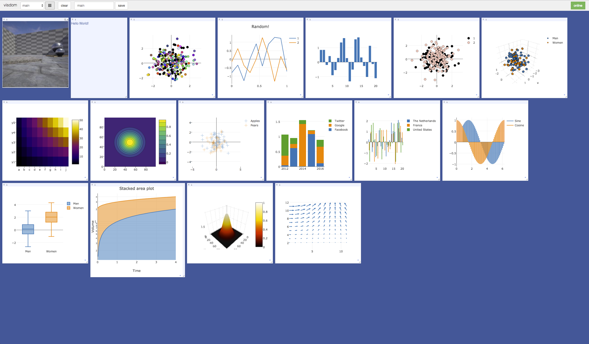
The UI begins as a blank slate – you can populate it with plots, images, and text. These appear in windows that you can drag, drop, resize, and destroy. The windows live in envs and the state of envs is stored across sessions. You can download the content of windows – including your plots in svg.
Tip: You can use the zoom of your browser to adjust the scale of the UI.
Callbacks
The python Visdom implementation supports callbacks on a window. The demo shows an example of this in the form of an editable text pad. The functionality of these callbacks allows the Visdom object to receive and react to events that happen in the frontend.
You can subscribe a window to events by adding a function to the event handlers dict for the window id you want to subscribe by calling viz.register_event_handler(handler, win_id, env=None) with your handler, the window id, and an optional environment name. Specifying the environment name prevents event handlers from firing across different environments with the same window id. Multiple handlers can be registered to the same window. You can remove event handlers from a window using viz.clear_event_handlers(win_id, env=None). When an event occurs to that window, your callbacks will be called on a dict containing:
- event_type: one of the below event types
- pane_data: all of the stored contents for that window including layout and content.
- eid: the current environment id
- target: the window id the event is called on
Additional parameters are defined below.
Right now the following callback events are supported:
Close- Triggers when a window is closed. Returns a dict with only the aforementioned fields.KeyPress- Triggers when a key is pressed. Contains additional parameters:
key - A string representation of the key pressed (applying state modifiers such as SHIFT)
- key_code - The javascript event keycode for the pressed key (no modifiers)
PropertyUpdate- Triggers when a property is updated in Property pane
propertyId - Position in properties list
- value - New property value
Click- Triggers when Image pane is clicked on, has a parameter:
image_coord - dictionary with the fields x and y for the click coordinates in the coordinate frame of the possibly zoomed/panned image (not the enclosing pane).
Editable Plot Parameters
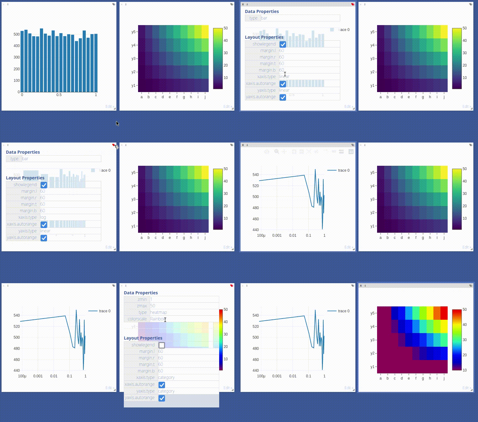
Use the top-right edit-Button to inspect all parameters used for plot in the respective window.
The visdom client supports dynamic change of plot parameters as well. Just change one of the listed parameters, the plot will be altered on-the-fly.
Click the button again to close the property list.
Environments

You can partition your visualization space with envs. By default, every user will have an env called main. New envs can be created in the UI or programmatically. The state of envs is persistently saved. Environments are able to keep entirely different pools of plots.
You can access a specific env via url: http://localhost:8097/env/main. If your server is hosted, you can share this url so others can see your visualizations too.
Environments are automatically hierarchically organized by the first _.
Note that / characters in environment names are escaped to _, so both _ and /
can affect how environments appear hierarchically in the UI.
Selecting Environments
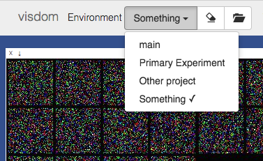
From the main page it is possible to toggle between different environments using the environment selector. Selecting a new environment will query the server for the plots that exist in that environment. The environment selector allows for searching and filtering for the new environment.
Comparing Environments
From the main page it is possible to compare different environments using the environment selector. Selecting multiple environments in the check box will query the server for the plots with the same titles in all environments and plot them in a single plot. An additional compare legend pane is created with a number corresponding to each selected environment. Individual plots are updated with legends corresponding to "x_name" where x is a number corresponding with the compare legend pane and name is the original name in the legend.
Note: The compare envs view is not robust to high throughput data, as the server is responsible for generating the compared content. Do not compare an environment that is receiving a high quantity of updates on any plot, as every update will request regenerating the comparison. If you need to compare two plots that are receiving high quantities of data, have them share the same window on a singular env.
Clearing Environments
You can use the eraser button to remove all of the current contents of an environment. This closes the plot windows for that environment but keeps the empty environment for new plots.Managing Environments
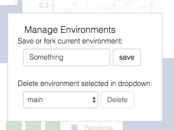
Pressing the folder icon opens a dialog that allows you to fork or force save the current environment, or delete any of your existing environments. Use of this feature is fully described in the State section.
Env Files:
Your envs are loaded upon request by the user, by default from$HOME/.visdom/. Custom paths can be passed as a cmd-line argument. Envs are removed by using the delete button or by deleting the corresponding.jsonfile from the env dir. In case you want the server to pre-load all files into cache, use the flag-eager_data_loading.
State
Once you've created a few visualizations, state is maintained. The server automatically caches your visualizations -- if you reload the page, your visualizations reappear.
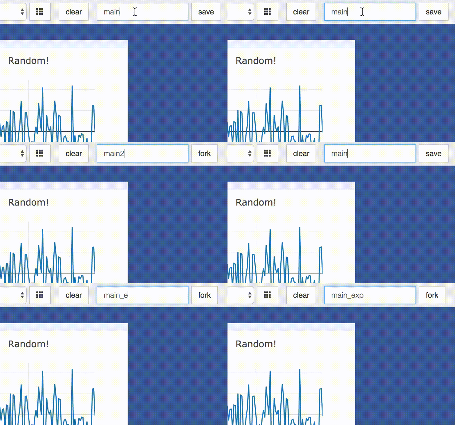
- Save: You can manually do so with the
savebutton. This will serialize the env's state (to disk, in JSON), including window positions. You can save anenvprogrammatically.
This is helpful for more sophisticated visualizations in which configuration is meaningful, e.g. a data-rich demo, a model training dashboard, or systematic experimentation. This also makes them easy to share and reuse.
- Fork: If you enter a new env name, saving will create a new env -- effectively forking the previous env.
Tip: Fork an environment before you begin to make edits to ensure that your changes are saved separately.
Filter
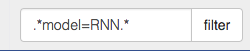
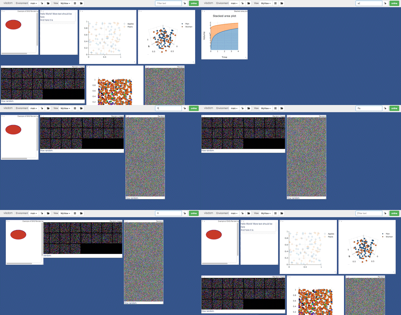
You can use thefilter to dynamically sift through windows present in an env -- just provide a regular expression with which to match titles of window you want to show. This can be helpful in use cases involving an env with many windows e.g. when systematically checking experimental results.
Note: If you have saved your current view, the view will be restored after clearing the filter.
Views

It is possible to manage the views simply by dragging the tops of windows around, however additional features exist to keep views organized and save common views. View management can be useful for saving and switching between multiple common organizations of your windows.
Saving/Deleting Views
Using the folder icon, a dialog window opens where views can be forked in the same way that envs can be. Saving a view will retain the position and sizes of all of the windows in a given environment. Views are saved in$HOME/.visdom/view/layouts.json in the visdom filepath.
Note: Saved views are static, and editing a saved view copies that view over to the current view where editing can occur.
Re-Packing
Using the repack icon (9 boxes), visdom will attempt to pack your windows in a way that they best fit while retaining row/column ordering.Note: Due to the reliance on row/column ordering and ReactGridLayout the final layout might be slightly different than what might be expected. We're working on improving that experience or providing alternatives that give more fine-tuned control.
Reloading Views
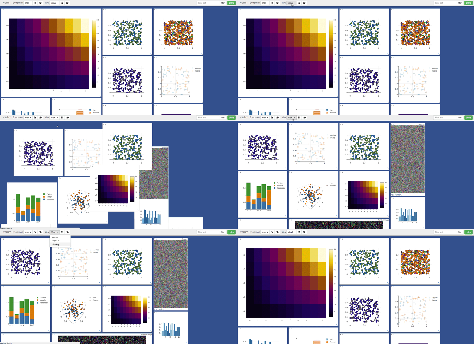
Using the view dropdown it is possible to select previously saved views, restoring the locations and sizes of all of the windows within the current environment to the places they were when that view was saved last.
Setup
Python and web clients come bundled with the python server.Install from pip
> pip install visdomInstall from source
> pip install git+https://github.com/fossasia/visdomOptional: To save Plotly figures to image files from code (e.g. PNG/SVG) without using the browser download button, install plotly and kaleido: pip install plotly kaleido. See vis.plotlyplot and vis.save_plotly_figure.
Usage
Start the server (probably in a screen or tmux) from the command line:
> visdomVisdom now can be accessed by going to http://localhost:8097 in your browser, or your own host address if specified.
Thevisdomcommand is equivalent to runningpython -m visdom.server.
If the above does not work, try using an SSH tunnel to your server by adding the following line to your local ~/.ssh/config:
``LocalForward 127.0.0.1:8097 127.0.0.1:8097`.
Command Line Options
The following options can be provided to the server:
-port : The port to run the server on.
-hostname : The hostname to run the server on.
-base_url : The base server url (default = /).
-env_path : The path to the serialized session to reload.
-logging_level : Logging level (default = INFO). Accepts both standard text and numeric logging values.
-readonly : Flag to start server in readonly mode.
-enable_login : Flag to setup authentication for the server, requiring a username and password to login.
-force_new_cookie : Flag to reset the secure cookie used by the server, invalidating current login cookies.Requires -enable_login.
-bind_local : Flag to make the server accessible only from localhost.
-eager_data_loading : By default visdom loads environments lazily upon user request. Setting this flag lets visdom pre-fetch all environments upon startup.
When -enable_login flag is provided, the server asks user to input credentials using terminal prompt. Alternatively,
you can setup VISDOM_USE_ENV_CREDENTIALS env variable, and then provide your username and password via
VISDOM_USERNAME and VISDOM_PASSWORD env variables without manually interacting with the terminal. This setup
is useful in case if you would like to launch visdom server from bash script, or from Jupyter notebook.
VISDOM_USERNAME=username
VISDOM_PASSWORD=password
VISDOM_USE_ENV_CREDENTIALS=1 visdom -enable_login
You can also use VISDOM_COOKIE variable to provide cookies value if the cookie file wasn't generated, or the
flag -force_new_cookie was set.
HTTPS Support
To run the visdom server over HTTPS,user need to provide an SSL certificate and key file:
# Generate a self-signed certificate (for development only)
openssl req -x509 -newkey rsa:4096 -keyout key.pem -out cert.pem -days 365 -nodes
Start the server with HTTPS
python -m visdom.server -ssl_certfile cert.pem -ssl_keyfile key.pem
Access the server at
https://localhost:8097.
Connect via the Python client:
# For Production - real CA-signed certificate (default)
vis = visdom.Visdom(server="https://myserver.com")
For Development - self signed certificate
vis = visdom.Visdom(server="https://localhost", ssl_verify=False)
Note:
ssl_verify=False disables certificate verification and should only be used in development with self-signed certificates. Do not use in production.
Python example
import visdom
import numpy as np
vis = visdom.Visdom()
vis.text('Hello, world!')
vis.image(np.ones((3, 10, 10)))
Demos
If you have cloned this repository, you can run our demo showcase.
python example/demo.py
The same showcase for the asyncio client — concurrent plots, a single-request append loop and a coroutine event handler — is in
example/async_demo.py; see Async usage.
python example/async_demo.py
API
For a quick introduction into the capabilities of visdom, have a look at the example directory, or read the details below.
Visdom Arguments (Python only)
The python visdom client takes a few options:
server: the hostname of your visdom server (default: 'http://localhost')
port: the port for your visdom server (default: 8097)
base_url: the base visdom server url (default: /)
env: Default environment to plot to when no env is provided (default: main)
raise_exceptions: Raise exceptions upon failure rather than printing them (default: True (soon))
log_to_filename: If not none, log all plotting and updating events to the given file (append mode) so that they can be replayed later using replay_log (default: None)
use_incoming_socket: enable use of the socket for receiving events from the web client, allowing user to register callbacks (default: True)
http_proxy_host: Deprecated. Use Proxies argument for complete proxy support.
http_proxy_port: Deprecated. Use Proxies argument for complete proxy support.
username: username to use for authentication, if server started with -enable_login (default: None)
password: password to use for authentication, if server started with -enable_login (default: None)
proxies: Dictionary mapping protocol to the URL of the proxy (e.g. {http: foo.bar:3128}) to be used on each Request. (default: None)
offline: Flag to run visdom in offline mode, where all requests are logged to file rather than to the server. Requires log_to_filename is set. In offline mode, all visdom commands that don't create or update plots will simply return True. (default: False)
use_preflight_checks: Ask the server whether a window exists before an update='append' or a store_history=True frame, which costs a second round trip per call. Set it to False to send one request and let the server create the window if it isn't there -- roughly halving the requests of an append loop. Requires a server new enough to lay out a window it creates from an append; against an older one such a window comes out unstyled. (default: True)
Other options are either currently unused (endpoint, ipv6) or used for internal functionality.
Async usage (Python only)
visdom.async_client.AsyncVisdom is an awaitable front end to the same client. It exists for callers that already run an event loop, or that want several plots in flight at once; visdom.Visdom is unchanged and remains the way to use visdom from ordinary synchronous code.
import asyncio
import numpy as np
from visdom.async_client import AsyncVisdom
async def main():
vis = await AsyncVisdom.create(server="http://localhost", port=8097)
async with vis:
await asyncio.gather(
vis.line(Y=np.random.rand(20), win="a"),
vis.line(Y=np.random.rand(20), win="b"),
)
asyncio.run(main())
Every plotting method of
Visdom is available with the same name, the same arguments and the same return value — as a coroutine. Nothing is reimplemented: the method bodies run as the synchronous code they already are, on a thread pool the client owns, and only the request itself is asynchronous. That is also why the CPU-heavy encodes (image, matplot) stay off your event loop for free.
Things to know:
- Build it with
create, not (). Connecting means a POST and __init__ cannot await. create accepts every Visdom argument, plus max_concurrency (default 10) which sizes both the client's thread pool and the number of requests tornado will start at once. max_concurrency only supplies the default for tornado's max_clients: pass max_clients explicitly and it wins, so the two limits then differ by as much as you asked for.
shutdown closes the client, close closes a window. close is Visdom.close and keeps its usual meaning, so the method that releases the HTTP client and the worker pool is shutdown(). Using the client as an async context manager calls it for you.
Two defaults differ from Visdom. use_incoming_socket is False here (most async callers never register a handler, and a backchannel costs a held-open connection plus a thread), and use_preflight_checks is False (an async client is new code talking to a server that understands layout_create, so an append costs one request rather than two). Pass either explicitly to get the synchronous behavior back.
Concurrency is yours to ask for. gather runs the calls on separate worker threads against one shared inner client, and that client is no more thread-safe than the synchronous one — concurrent calls should target distinct windows.
Event handlers work, and may be coroutines. Pass use_incoming_socket=True (or use_polling=True for the HTTP fallback) and register as usual with register_event_handler; registration is not a coroutine, since it never reaches the server. A plain handler runs on the client's own single dispatch thread; a coroutine handler has only its wrapper there, and its body runs on your loop, so it can await further calls on the same client. Either way handlers run one at a time, in arrival order.
No HTTP proxies. create raises NotImplementedError for proxies / http_proxy_host / http_proxy_port: the transport is tornado's AsyncHTTPClient, which has no proxy support without pycurl. Use Visdom behind a proxy.
Measured on loopback over 300 line(update='append') calls — the path profiled in #771:
| Client | plots/s | p50 | p95 |
|---|---|---|---|
|
Visdom, preflight on (default) | 198 | 5.00 ms | 5.73 ms |
| Visdom, use_preflight_checks=False | 304 | 3.32 ms | 4.09 ms |
| AsyncVisdom, awaited serially | 235 | 4.24 ms | 4.87 ms |
| AsyncVisdom, 8 concurrent | 410 | 13.19 ms | 18.33 ms |
Requests halve exactly once the preflight is off. Throughput does not quite double because on loopback the preflight is the cheaper of the two round trips; over a real network the two cost the same.
example/async_demo.py runs all of the above against a live server.
Basics
Visdom offers the following basic visualization functions:
vis.image : image
vis.image_heatmap : image with heatmap overlay
vis.update_image_slider : set visible frame of an image_history pane
vis.images : list of images
vis.text : arbitrary HTML
vis.properties : properties grid
vis.table : editable, resizable table pane
vis.html_table : static styled HTML table
vis.audio : audio
vis.video : videos
vis.svg : SVG object
vis.matplot : matplotlib plot
vis.plotlyplot : arbitrary Plotly figure
vis.embeddings : interactive embedding projection
vis.save : serialize state server-side
Plotting
We have wrapped several common plot types to make creating basic visualizations easily. These visualizations are powered by Plotly.
The following API is currently supported:
vis.scatter : 2D or 3D scatter plots
vis.sunburst : sunburst (hierarchy) charts
vis.line : line plots
vis.learning_curve : named training metric curves
vis.stem : stem plots
vis.heatmap : heatmap plots
vis.confusion_matrix : confusion matrix plots
vis.bar : bar graphs
vis.histogram : histograms
vis.histogram2d : 2D histograms (density maps)
vis.boxplot : boxplots
vis.violin : violin plots
vis.pie : pie charts
vis.surf : surface plots
vis.contour : contour plots
vis.roc_curve : ROC curves
vis.pr_curve : precision-recall curves
vis.quiver : quiver plots
vis.mesh : mesh plots
vis.sankey : sankey (flow) diagrams
vis.dual_axis_lines : double y axis line plots
vis.graph : network graphs
Generic Plots
Note that the server API adheres to the Plotly convention of data and layout objects, such that you can produce your own arbitrary Plotly visualizations:
import visdom
vis = visdom.Visdom()
trace = dict(x=[1, 2, 3], y=[4, 5, 6], mode="markers+lines", type='custom',
marker={'color': 'red', 'symbol': 104, 'size': "10"},
text=["one", "two", "three"], name='1st Trace')
layout = dict(title="First Plot", xaxis={'title': 'x1'}, yaxis={'title': 'x2'})
vis._send({'data': [trace], 'layout': layout, 'win': 'mywin'})
Others
vis.close : close a window by id
vis.delete_env : delete an environment by env_id
vis.win_exists : check if a window already exists by id
vis.get_env_list : get a list of all of the environments on your server
vis.get_window_data: get current data for a window
vis.set_tags: replace or append environment tags
vis.get_tags: read environment tags
vis.save_plotly_figure: save a Plotly figure to an image file from code (no browser click)
vis.check_connection: check if the server is connected
vis.replay_log: replay the actions from the provided log file
Experiments
Track experiment metadata (hyper-parameters, metrics, tags) alongside your plots, then search and compare runs across your server:
vis.experiment : create or update experiment metadata for an env
vis.log_metrics : append metric observations to an env's experiment
vis.finish_experiment : mark an experiment terminal (finished/failed)
vis.search_experiments : search experiments across envs with a query
vis.compare_experiments : diff experiments field by field
vis.suggest_experiment : suggest parameters for the next run (reserved)
vis.hparams : open a hyper-parameter pane over the selected runs
vis.update_hparams : change or refresh an existing hyper-parameter pane
Loggers
Framework-specific logging bridges that wrap the Visdom API so training loops stay focused on training. Each logger lives in its own submodule and handles window creation, step tracking, and throttling internally. None of the framework packages below are part of Visdom's own install — each logger imports its framework lazily and raises a clear
ImportError with the pip install command if it's missing.
PyTorch
Requirements:
pip install visdom torch
visdom.pytorch.VisdomLogger is a context manager for raw PyTorch training loops. Call tracker.log(name, value) for any scalar — no viz.line() arguments needed.
Epoch-level logging (recommended default — one call per epoch):
import visdom
from visdom.pytorch import VisdomLogger
viz = visdom.Visdom()
with VisdomLogger(viz, env="my_run") as tracker:
for epoch in range(num_epochs):
train_loss = run_train_epoch(model, loader)
val_loss = run_val_epoch(model, val_loader)
tracker.log("Train Loss", train_loss)
tracker.log("Val Loss", val_loss)
tracker.log("LR", optimizer.param_groups[0]["lr"])
Per-batch logging with
log_every — use when logging inside the batch loop on large datasets:
with VisdomLogger(viz, env="my_run", log_every=50) as tracker:
for epoch in range(num_epochs):
for inputs, targets in train_loader:
loss = criterion(model(inputs), targets)
optimizer.zero_grad()
loss.backward()
optimizer.step()
# sent to Visdom every 50 batches, not every batch
tracker.log("Train Loss", loss.item(), xlabel="step")
tracker.log("LR", optimizer.param_groups[0]["lr"], xlabel="step")
Experiment tracking with
params — pass hyperparameters to also record the run as a queryable experiment, alongside the usual charts:
params = {"lr": 1e-2, "batch_size": 32}
with VisdomLogger(viz, env="my_run", params=params) as tracker:
for epoch in range(num_epochs):
tracker.log("Train Loss", train_loss)
later, from anywhere
viz.search_experiments("lr < 0.01 AND status = finished")
viz.compare_experiments(["my_run", "my_other_run"])
Tracking is opt-in: without
params, VisdomLogger only ever calls viz.line(), unchanged from before this existed. With params, the run's status is recorded as finished on a normal exit or failed if the with-block raised, and every logged metric is mirrored into the experiment alongside the chart it's plotted on.
Parameters:
viz: a connected visdom.Visdom() instance
env: environment name (default: auto-generated from timestamp)
log_every: send every N calls per metric — use with per-batch logging on large datasets (default: 1)
params: dict of hyperparameters; opts into experiment tracking (default: None, tracking off)
Each unique name passed to tracker.log() gets its own window. The first call creates it; subsequent calls append. See example/train_example.py for a full working example.
PyTorch Lightning
Requirements:
pip install visdom lightning (or pip install visdom pytorch-lightning)
visdom.loggers.VisdomLightningLogger implements Lightning's Logger protocol. Lightning aggregates every self.log() / self.log_dict() call in a LightningModule and hands the result to the logger, so nothing in the model or training loop changes — the user passes one logger= argument to Trainer.
import lightning.pytorch as pl
import visdom
from visdom.loggers import VisdomLightningLogger
viz = visdom.Visdom()
logger = VisdomLightningLogger(viz, env="lightning_run")
trainer = pl.Trainer(max_epochs=20, logger=logger, log_every_n_steps=5)
trainer.fit(model, train_loader, val_loader)
Each metric key gets its own window — one key, one line chart, with no train/val name parsing. The
epoch key Lightning mixes into the metrics dict is not plotted. How often the logger is called is controlled by Lightning (Trainer(log_every_n_steps=...) for step metrics, once per epoch for epoch metrics).
Hyperparameters passed to
self.save_hyperparameters() are rendered once as a properties pane via viz.properties().
Gradient norms come from Lightning, not the logger. Add to your
LightningModule and they arrive through the logger like any other metric:
from lightning.pytorch.utilities import grad_norm
def on_before_optimizer_step(self, optimizer):
self.log_dict(grad_norm(self, norm_type=2))
Parameters:
viz: a connected visdom.Visdom() instance
env: environment name (default: viz.env if set, otherwise auto-generated from timestamp)
Note: each call to viz.line() is a synchronous network request made on the thread Lightning calls from, so a very small log_every_n_steps with many metrics can stall training while it waits on the server.
Note:
log_metrics and log_hyperparams run on rank zero only. Use one logger instance per Trainer run. Not thread-safe — internal state has no locking.
Note: when the run ends (success or failure) the logger saves the env on the server, so it can be reloaded later.
Note: values that don't convert to a float (non-numeric strings, multi-element tensors,
None) are skipped with a warning rather than raising.
See
example/train_lightning_example.py for a full working example.
scikit-learn
Requirements:
pip install visdom scikit-learn
visdom.loggers.VisdomSklearnLogger patches all sklearn fit() calls so every estimator trained after autolog() logs to Visdom automatically — no per-estimator code needed.
Plain estimators (classifiers, regressors, clusterers) produce a text pane with the estimator name, dataset shape, training score, fit time, and all hyperparameters.
GridSearchCV / RandomizedSearchCV produce a bar chart of
mean_test_score per parameter combination and a text pane with best_score_, best_params_, and fit time.
Iterative estimators additionally get a line chart of their per-iteration training history:
MLPClassifier/MLPRegressor plot loss_curve_ (plus validation_scores_ when fit with early_stopping=True), and GradientBoostingClassifier/GradientBoostingRegressor plot train_score_.
Regressors get
train_rmse and train_mae rows in the text pane alongside the R2 train_score (R2 alone can be misleading), plus a predicted-vs-residual scatter plot.
Note:
train_score, train_rmse, train_mae and the residual scatter are all measured on the data passed to fit(). They describe fit quality on the training set and are not held-out estimates — score your own test set for that.
Note: panes are keyed on the estimator instance, so refitting the same estimator updates the panes it already owns instead of opening new ones. Two different estimator objects always get their own panes, even of the same class.
Note: one logger is active at a time. Calling
autolog() again switches the active env silently — no warning is raised, and the previous env stops receiving updates.
import visdom
from visdom.loggers import VisdomSklearnLogger
from sklearn.ensemble import RandomForestClassifier
from sklearn.linear_model import Ridge
from sklearn.model_selection import GridSearchCV
viz = visdom.Visdom()
VisdomSklearnLogger.autolog()
clf = RandomForestClassifier(n_estimators=100)
clf.fit(X_train, y_train) # -> text pane
reg = Ridge(alpha=1.0)
reg.fit(X_train, y_train) # -> text pane
gs = GridSearchCV(clf, param_grid, cv=3)
gs.fit(X_train, y_train) # -> bar chart + text pane
If you have a custom Visdom connection (non-default port, remote server, auth), pass it explicitly:
import visdom
viz = visdom.Visdom(port=8098, server="http://myserver")
VisdomSklearnLogger.autolog(viz, env="sklearn_run")
Parameters:
viz: a connected visdom.Visdom() instance (optional — created internally if not passed)
env: environment name (default: viz.env if set, otherwise auto-generated from timestamp)
See example/train_sklearn_example.py for a full working example covering plain estimators and grid search.
XGBoost
Requirements:
pip install visdom xgboost
visdom.loggers.VisdomXGBLogger implements XGBoost's TrainingCallback protocol, plotting train/eval metrics to Visdom after every boosting round.
There was no way to visualize XGBoost training runs in Visdom without manually attaching a
TrainingCallback and wiring up viz.line() calls yourself. This adds opt-in auto-logging behind a single autolog() call, with no changes required to model, train(), or fit() code.
import xgboost as xgb
import visdom
from visdom.loggers import VisdomXGBLogger
viz = visdom.Visdom()
VisdomXGBLogger.autolog(viz, env="xgb_run")
booster = xgb.train(params, dtrain, evals=[(dtrain, "train"), (dval, "eval")]) # logged automatically
clf = xgb.XGBClassifier().fit(X_train, y_train, eval_set=[(X_val, y_val)]) # logged automatically
xgb.cv(params, dtrain, nfold=3) # logged automatically
Or attach a logger to a single run without patching anything:
callback = VisdomXGBLogger(viz, env="xgb_run")
booster = xgb.train(params, dtrain, evals=[(dtrain, "train"), (dval, "eval")], callbacks=[callback])
Each eval metric gets its own window with one trace per data name (
train/eval), and best_iteration/best_score are logged as a text pane once training finishes. See example/train_xgboost_example.py for a full working example.
Note: one logger is active at a time. Calling
autolog() again for a different env moves logging there and warns; the previous env keeps the windows it already has. Import cross_validate after autolog() — importing it first binds the original function, and every fold then opens its own window instead of sharing one per metric.
TensorFlow / Keras
Requirements:
pip install visdom tensorflow (or pip install visdom keras)
visdom.loggers.VisdomKerasLogger implements Keras's Callback protocol, plotting train/val metrics to Visdom after every epoch.
from tensorflow import keras
from tensorflow.keras import layers
import visdom
from visdom.loggers import VisdomKerasLogger
viz = visdom.Visdom()
logger = VisdomKerasLogger(viz, env="keras_run")
model = keras.Sequential([
layers.Input(shape=(20,)),
layers.Dense(32, activation="relu"),
layers.Dense(1, activation="sigmoid"),
])
model.compile(optimizer="adam", loss="binary_crossentropy", metrics=["accuracy"])
model.fit(
x_train, y_train,
validation_data=(x_val, y_val),
epochs=20,
callbacks=[logger],
)
A metric named
val_ is plotted as a val trace on the same window its train counterpart plots as a train trace, matching how Keras already splits train/val by key prefix. One instance can be reused across multiple fit() calls — a new run's epoch 0 replaces the previous run's curve on the same windows in place, rather than opening a duplicate set of windows.
Per-batch logging with
log_every — use when you also want step-level detail on large datasets. Off by default, since on_train_batch_end otherwise fires every batch regardless of whether step-level detail is wanted:
logger = VisdomKerasLogger(viz, env="keras_run", log_every=50)
model.fit(x_train, y_train, epochs=20, callbacks=[logger])
Each metric gets its own window titled
", throttled to one send every log_every batches. The optimizer's current learning rate is read (not computed) and plotted alongside as lr.
Experiment tracking with
params — records the run in the ExperimentStore alongside the charts, so it becomes queryable through vis.search_experiments / vis.compare_experiments. Off by default. Without params the logger only ever calls viz.line():
logger = VisdomKerasLogger(viz, env="keras_run", params={"lr": 0.01})
model.fit(x_train, y_train, epochs=20, callbacks=[logger])
viz.search_experiments("status = finished")
Hyper-parameters are recorded when training begins, each epoch's metrics as they are plotted, and the run is marked
finished when fit() returns. Only epoch metrics are recorded — per-batch values from log_every stay visualization-only so a run's metric history keeps the granularity the search and compare views read it at.
Note: a finished experiment rejects further writes, so an env records one tracked run. Give every run its own env, including a repeat run of the same script. Keras reports no exception to
on_train_end, so a tracked run is always recorded as finished. Call viz.finish_experiment(status="failed", env=...) directly to record a run that did not.
Parameters:
viz: a connected visdom.Visdom() instance
env: environment name (default: viz.env if set, otherwise auto-generated from timestamp)
log_every: also plot metrics at batch granularity, one send every N batches (default: None, disabled)
params: hyper-parameters to record, opting the run into experiment tracking (default: None, disabled)
Note: each call to viz.line() is a synchronous network request made on the training thread. Pick a log_every large enough that it doesn't stall training waiting on the server — 50+ is a reasonable default on GPU.
Note: not thread-safe — internal state has no locking, so calling
fit() on the same logger instance from multiple threads can race.
See
example/train_keras_example.py for a full working example.
Optuna
Requirements:
pip install visdom optuna
Dashboard visualizations:
pip install plotly
visdom.integrations.OptunaCallback implements Optuna's study callback
protocol. After each trial finishes it records the trial's parameters, objective
values and state as a Visdom experiment in a dedicated environment. Optuna is
not a Visdom dependency, so existing Visdom users do not install it unless they
choose this integration.
import optuna
import visdom
from visdom.integrations import OptunaCallback
viz = visdom.Visdom()
callback = OptunaCallback(
viz,
dashboard_env="optuna_quadratic",
objective_names=["loss"],
create_dashboard=True,
refresh_every=10,
contour_params=["x", "y"],
)
def objective(trial):
x = trial.suggest_float("x", -10, 10)
y = trial.suggest_float("y", -10, 10)
return (x - 2) 2 + (y + 1) 2
study = optuna.create_study(study_name="quadratic", direction="minimize")
study.optimize(objective, n_trials=100, callbacks=[callback])
callback.update_dashboard(study)
For multi-objective studies, list the objective names in the same order as the
study directions and return values:
callback = OptunaCallback(
viz,
dashboard_env="optuna_accuracy_latency",
objective_names=["accuracy", "latency_ms"],
create_dashboard=True,
)
def multi_objective(trial):
width = trial.suggest_int("width", 1, 10)
accuracy = 0.80 + 0.01 * width
latency_ms = 10.0 + 2.0 * width
return accuracy, latency_ms
study = optuna.create_study(
study_name="accuracy-latency",
directions=["maximize", "minimize"],
)
study.optimize(multi_objective, n_trials=40, callbacks=[callback])
callback.update_dashboard(study)
The integration records one experiment per trial, using names such as
optuna_quadratic_trial_000017. Intermediate values reported with
trial.report(value, step) are stored as the intermediate_value metric in
step order before the final objective value. Each experiment also carries a
stable optuna_dashboard_env tag. With create_dashboard=True, the first trial
creates summary, HParams, optimization history and timeline panes, plus
intermediate-value and parameter-importance panes when Optuna can compute them.
Supplying at least two parameter names through contour_params adds a contour
pane for each objective; Optuna handles numerical, categorical and log-scaled
parameters when it builds those Plotly figures.
The HParams pane selects experiments by that dashboard tag rather than by a
callback-local list, so update_dashboard() on a new callback recovers trials
logged before a process restart. Dashboard refreshes from one callback are
serialized, so study.optimize(..., n_jobs=N) cannot publish them out of order.
When multiple processes or nodes share a study and dashboard namespace, enable
create_dashboard=True in exactly one process; callbacks in the other workers
still log their trials with the default create_dashboard=False. The designated
writer's tag query includes trials from every worker. After all workers finish,
have the coordinating process call update_dashboard() once for the final
refresh.
Completed studies with two or three objectives also get a Pareto-front pane.
Later trials refresh the panes in
optuna_quadratic every refresh_every
successful writes by the dashboard writer. The explicit final
update_dashboard() includes any trials left since the last scheduled refresh.
Plotly is only needed for the Optuna visualization panes. Timeline bars preserve
each trial's true duration, and a fixed-size marker at the true start time keeps
even sub-pixel trials visible and hoverable without exaggerating their runtime.
The summary pane links directly to the best and latest terminal trial
environments. The callback never opens a browser on its own.
Pass
raise_on_error=True if a Visdom logging failure should stop optimization;
by default it emits a warning and allows the study to continue. Single- and
multi-objective studies are supported, and COMPLETE, PRUNED and FAIL
states are preserved in the optuna_state tag. A pruned trial retains every
intermediate value reported before pruning. Optuna remains responsible for the
pruning decision: call trial.report() and trial.should_prune() inside the
objective and raise optuna.TrialPruned when requested. Because Optuna invokes
study callbacks after a trial reaches a terminal state, OptunaCallback
records these values after the trial finishes rather than streaming them while
the trial is running. Optuna does not support
trial.report() or
trial.should_prune() for multi-objective studies, so intermediate-value and
pruning support applies only to single-objective studies.
Details
Basics
vis.image
This function draws an img. It takes as input an CxHxW tensor img that contains the image.
Most Python image libraries (e.g. OpenCV, PIL, matplotlib) return images in HxWxC format.
Passing images in that format will raise errors or lead to incorrect rendering.
For example:
# Convert HxWxC → CxHxW before passing to vis.image
img = img.transpose(2, 0, 1) # NumPy
img = img.permute(2, 0, 1) # PyTorch
The following
opts are supported:
jpgquality: JPG quality (number 0-100). If defined image will be saved as JPG to reduce file size. If not defined image will be saved as PNG.
caption: Caption for the image
store_history: Keep all images stored to the same window and attach a slider to the bottom that will let you select the image to view. You must always provide this opt when sending new images to an image with history.
vis.update_image_slider
Programmatically set the visible frame of an
image_history pane from Python:
win = vis.image(img, opts=dict(store_history=True))
vis.image(img2, win=win, opts=dict(store_history=True))
vis.update_image_slider(win, index=1) # show second frame
The
index is 0-based and is clamped to the valid range by the server. NumPy integer scalars (e.g. np.int64) are accepted and coerced automatically. Passing a non-integer or a non-image_history window raises an error.
Note You can use alt on an image pane to view the x/y coordinates of the cursor. You can also ctrl-scroll to zoom, alt scroll to pan vertically, and alt-shift scroll to pan horizontally. Double click inside the pane to restore the image to default.
vis.image_heatmap
This function overlays a saliency or attention heatmap on top of an image. It takes a
CxHxW or HxW array img (uint8 or float) and an HxW float array heatmap with values in [0, 1]. The blending is per-pixel — pixels where the heatmap is near zero stay close to the original image, so a zero-gradient background does not get tinted by the colormap.
import numpy as np
from visdom import Visdom
viz = Visdom()
img: CxHxW uint8 or float in [0, 1]
heatmap: HxW float in [0, 1] — e.g. from a saliency method or attention map
viz.image_heatmap(img, heatmap, opts=dict(title="Saliency", alpha=0.6, colormap="jet"))
Any attribution method that produces an
HxW numpy array works — gradient saliency, GradCAM, SHAP, or a hand-computed attention map.
The following
opts are supported:
alpha: blend strength (float in [0, 1]; default = 0.5). Higher values make the heatmap more visible.
colormap: matplotlib colormap name (string; default = 'jet'). Falls back to a blue-red gradient if matplotlib is not installed.
caption: caption for the image pane
jpgquality: JPG quality (number 0-100). If set, the result is encoded as JPEG. Otherwise PNG.
normalize: normalize the image to [0, 1] before blending (boolean; default = False)
Note
heatmap accepts any finite float range. Values outside [0, 1] are rescaled automatically via min-max normalization, so methods like SHAP or Integrated Gradients that return signed or unnormalized values work without any pre-processing. NaN maps to 0; infinite values are clamped to the [0, 1] boundary.
vis.images
This function draws a list of
images. It takes an input B x C x H x W tensor or a list of images all of the same size. It makes a grid of images of size (B / nrow, nrow).
The following arguments and
opts are supported:
nrow: Number of images in a row
padding: Padding around the image, equal padding around all 4 sides
opts.jpgquality: JPG quality (number 0-100). If defined image will be saved as JPG to reduce file size. If not defined image will be saved as PNG.
opts.caption: Caption for the image
vis.text
This function prints text in a box. You can use this to embed arbitrary HTML.
It takes as input a text string.
No specific opts are currently supported.
vis.properties
This function shows editable properties in a pane. Properties are expected to be a List of Dicts e.g.:
``
properties = [
{'type': 'text', 'name': 'Text input', 'value': 'initial'},
{'type': 'number', 'name': 'Number input', 'value': '12'},
{'type': 'button', 'name': 'Button', 'value': 'Start'},
{'type': 'checkbox', 'name':
... (README truncated for length)