
TL;DR
When DeepSeek-V4.1 Flash was released, I thought it might just be a post-training iteration version... but after using it for a while, I found it reached nearly 420 Tokens/s in speed, and then Cui said all DeepSeek-V4 Pro models would be taken offline... suddenly I felt this was no small matter... until the Technical Report 《DeepSeek-V4.1-Flash: Pushing the Limits of KV Cache Compression》[1] was fully released, only then did I realize it should be called DeepSeek-V5 Flash...
As the paper title states, the purpose of DeepSeek-V4.1 Flash is to push KVCache compression to the extreme. The main reason is that Long-horizon Agent Workflows cause the Context to grow longer and longer, while various tool calls bring heavy prefill computation pressure. The storage pressure of KVCache in HBM and external SSD is very high, all of which are reasons that make Scaling impossible. Therefore, a series of optimizations were made on the model architecture, especially in the compression of KVCache and the computation optimization of Prefill.
Prefill computation optimization: Drawing on YOCO, the entire model has 40 layers, and only 20 layers are needed during Prefill. Therefore, the Prefill activated parameters are only 8B, and the Decode activated parameters are 16B KVCache compression: Engineering-wise, KVCache compression is divided into several dimensions: head count compression similar to GQA, then block-based compression like CSA, and the cross-layer compression of CSA2 in this paper. At the same time, the indexer computation of Sparse Attention is also optimized. Finally, there are some numerical precision optimizations, for example DS41F adopts FP4 KVCache.
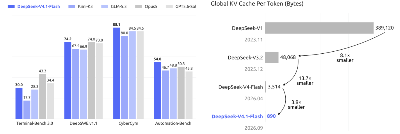
Finally, under the premise of maintaining high-quality task completion by the model, KVCache is further compressed by 4x:
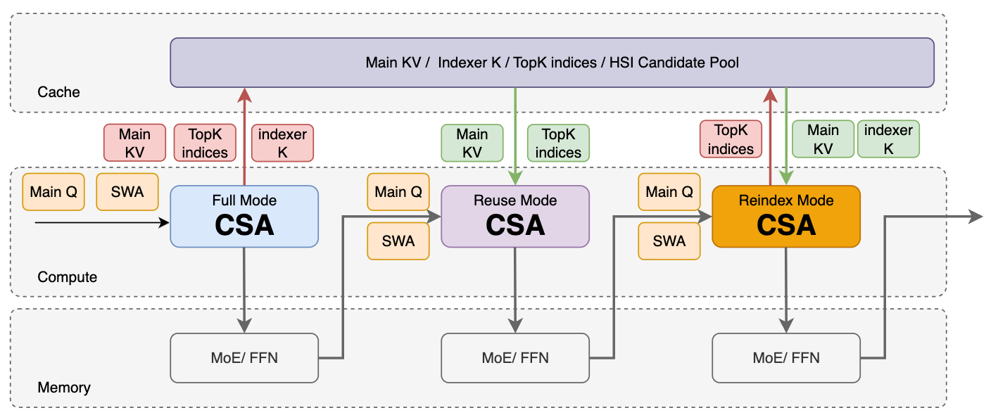
In addition, the original writing of the paper is somewhat complex, especially the description of CED. In fact, if we redraw a diagram centered on KVCache and combined with the perspective of computer architecture, it seems to become clear all at once. It can be seen as a kind of Recursive Transformer architecture, a way of modifying Q and reusing KV during the recursive process.
Regarding the Recursive Transformer architecture, you can refer to 《On the Future Transformer: Loops Are Not What You Need》. Next, we will conduct a detailed interpretation and analysis according to the chapter structure of the technical report. This article is the first in this series, analyzing the model architecture in detail, and the more critical content is in Chapter 3.
1. Overview
1.1 Why KVCache compression is needed
First, the report states that in recent years Long-horizon Agents have made ultra-long-context processing an increasingly important model workload. Supporting this type of workload not only requires efficient processing of long sequences, but also requires persistent storage, reuse, and transfer of large KVCache. Therefore, KVCache management has become a fundamental capability of model deployment, while also bringing significant challenges in computation, storage, and communication.
Then it goes on to introduce the DeepSeek-V4 architecture, which processes by combining a Sparse Attention that fully covers the context with a Sliding Window Attention (SWA) that covers the local window. Although advances related to Sparse Attention have significantly reduced the computational cost of long sequence processing, persistent storage and data movement have gradually become more prominent bottlenecks. In long contexts, the usage of the Global KV Cache will dominate, and being persisted for prefix reuse, it will heavily occupy Host memory capacity and SSD capacity, and will also place high demands on the interconnect bandwidth for KVCache movement. These limit service throughput, increase deployment cost, and ultimately hinder the deployment and promotion of agents toward longer task spans and broader application scenarios.
Therefore, further reducing the key-value cache footprint is crucial for alleviating storage and communication bottlenecks and reducing long-context serving costs. DeepSeek-V4.1-Flash is a multimodal mixture-of-experts model designed for more aggressive KVCache compression. DeepSeek-V4.1-Flash has a parameter scale of 552B, natively supports multimodal input, and supports contexts of up to 1 million tokens. It adopts a Causal Encoder-Decoder (CED) architecture, in which the Decoder's Global KVCache is obtained by projecting the Encoder's final hidden states. This design makes the model activate 8B parameters per token during the Prefill stage and 16B parameters during the Decoding stage, which is especially cost-effective for input-dominated Agent scenarios. Although DeepSeek-V4.1-Flash is significantly larger than DeepSeek-V4-Flash, at the same sequence length, its required runtime KVCache storage is only about 1/4 of the latter, and its persistent KVCache storage is only about 1/8 of the latter. In addition, the overall performance of DeepSeek-V4.1-Flash is superior to DeepSeek-V4-Flash.
These compressions for KVCache mainly come from the joint optimization of model architecture, cache precision, and deployment strategy. For DSv4, it is a model with SWA as the backbone and enhanced by global compressed attention (CSA/HCA). Based on this perspective, the DeepSeek team carried out a series of optimizations. First, it is worth noting that they abandoned the block-based high-compression-ratio structure like HCA, and instead carried out more optimizations on CSA, forming CSA2. The main optimizations compress the KV Cache from three dimensions:
In the channel dimension, a 512-dimensional latent vector is used to share the representation of the keys and values required by each attention head; In the sequence dimension, the Encoder merges 2 adjacent positions into 1 cache entry through channel-wise learned weights, while the Decoder retains per-position entries; In the layer dimension, multiple layers share the same global KV, and the whole network retains only 3 copies of Encoder cache and 1 copy of Decoder cache.
Combined with FP4 quantization, the storage growth of the global main KV and the Indexer is about 890 bytes per token.
1.2 Overview of model architecture
The overall model architecture is as follows:
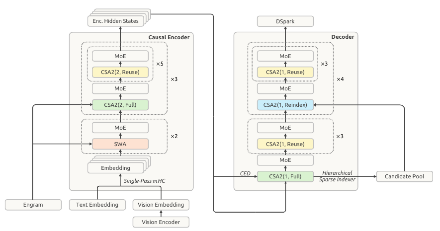
The paper reports that the backbone parameters are about , the Engram parameters are about , and the activated parameters per token for prefill and decode are about and respectively. The core is to use CED to reduce long-context Prefill computation, use CSA2 to reduce attention and KV cache overhead, and then combine Engram conditional memory with DSpark speculative decoding.
The model has layers in total, hidden dimension , and vocabulary size . Each layer contains attention and MoE, organized through mHC residual connections. The entire attention mechanism is divided into two modules, Encoder and Decoder, forming a Causal Encoder-Decoder (CED) architecture. The key of CED is that the Decoder's global KV comes from the Encoder's end representation, and subsequent Decoder layers share these KVs. Therefore, most positions of a long prompt only need to pass through the first 20 layers,
The key CSA2 among them adopts a mechanism of local sliding window + global sparse retrieval + cross-layer KVCache reuse. The sliding window size is 128, attention uses Q heads, sharing a -dimensional KV latent, of which RoPE is -dimensional and NoPE is -dimensional. Q uses a low-rank projection of rank , and the output projection is divided into groups, each of rank . The relevant parameters of the entire model are as follows:
| Category | Field | Value | Meaning |
|---|---|---|---|
| Backbone | dim |
5120 | Hidden dimension |
n_layers |
40 | First 20 layers are Encoder Last 20 layers are Decoder |
|
n_mtp_layers |
3 | DSpark three SWA-128 blocks | |
vocab_size |
129280 | — | |
| Attention | n_heads |
64 | |
head_dim |
512 | Latent dimension | |
rope_head_dim |
64 | RoPE component dimension NoPE component |
|
q_lora_rank |
1280 | ||
o_lora_rank /o_groups |
1024 / 8 | Output projection divided into 8 groups, each of rank 1024 | |
window_size |
128 | SWA sliding window | |
| CSA2 | compress_ratios |
[0,0, 2×18, 1×20, 0,0,0] |
Encoder layer compression ratio is 2 Decoder layer compression ratio is 1 |
kv_source_layers |
[2,8,14,20] |
Full mode layers | |
index_source_layers |
[2,8,14,20,24,28,32,36] |
Full + Reindex mode layers | |
index_n_heads /index_head_dim |
32 / 128 | indexer scale | |
index_topk |
512 | Top-K count | |
candidate_source_layer |
20 | Candidate pool construction layer | |
candidate_topk_blocks /candidate_block_size |
2048 / 8 | candidates | |
| RoPE | original_seq_len |
65536 | |
rope_factor |
16 | ||
rope_theta /compress_rope_theta |
10000 / 160000 | ||
| MoE | n_routed_experts /n_activated_experts |
384 / 6 | Top-6 of 384 |
moe_inter_dim |
2304 | Expert intermediate dimension | |
score_func |
sqrtsoftplus |
Continues to use sqrtsoftplus | |
route_scale /swiglu_limit |
1.5 / 10.0 | — | |
| mHC | hc_mult |
4 | residual streams |
hc_sinkhorn_iters |
20 | sk iterated 20 times | |
| Engram | engram_layer_ids |
[1, 14] |
Injected at layer 1 and layer 14 |
engram_num_embeddings |
[384006168, 384016682] |
Number of rows of the two tables | |
engram_max_ngram_size /engram_n_heads |
4 / 8 | N-gram orders , 8 heads | |
engram_head_dim |
256 | , total embedding dimension per order 2048 |
|
engram_vocab_size |
16000000 | About 16M entries | |
| DSpark | dspark_block_size |
5 | Draft |
dspark_target_layer_ids |
[37,38,39] |
||
dspark_n_routed_experts |
128 | Draft layers use a smaller MoE | |
| Vision | vision_n_layers / vision_dim |
32 / 1024 | — |
vision_patch_size /vision_downsample_ratio |
14 / 3 | 3×3 downsampling → 9x token reduction | |
vision_max_n_token |
1024 | Token upper limit per single image |
Among them:
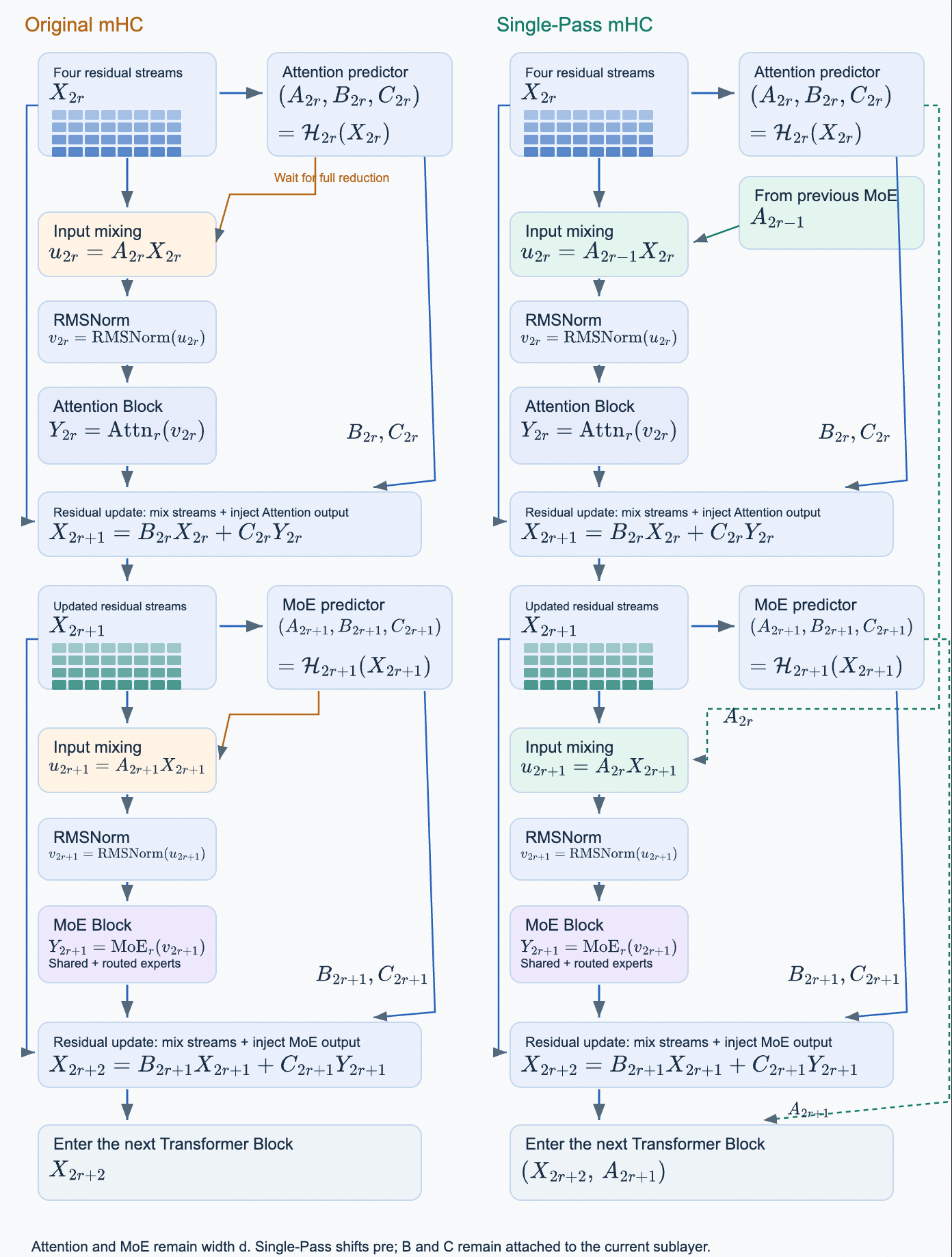
mHC: Each token maintains residual streams of dimensions. The residual mixing matrix is constrained to an approximately doubly stochastic matrix through Sinkhorn iterations. The key of Single-Pass is to use the input mixing coefficients produced by the previous sub-layer, releasing the dependency of the current coefficient computation, facilitating kernel fusion and reducing memory read/write. DSpark: An additional SWA-128 draft blocks, each layer adopts a small-scale MoE with Top-3 out of routed experts. It reads the mean of the four residual streams at the entry of backbone network layers , computes draft positions in parallel at once, cooperates with a Markov head to model dependencies, and a confidence head assists in deciding the verification length. Vision branch: A ViT with layers and hidden dimension , patch size . Features go through pixel-unshuffle, reducing the number of tokens to of the original, then mapped to dimensions by an MLP and inserted into the text sequence, with a maximum of visual tokens per single image.
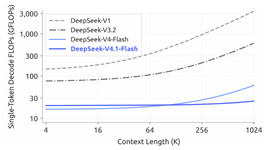
Regarding CED and CSA2, we will introduce them in detail in Chapter 2. Finally, as the Context grows, the required computation of DeepSeek V4.1 Flash grows almost linearly within the 1M range, and the computation overhead is far less than that of previous generations of models
2. Model Architecture
2.1 Multimodal architecture
The visual path of DeepSeek-V4.1-Flash can be summarized as: complete visual encoding on a finer image patch grid, rearrange adjacent features into fewer wide vectors, and then project them into the input space of the language backbone. Among them:
vision_patch_size=14: is the patch size of the original imagevision_downsample_ratio=3: is the merging range of the ViT output feature grid
The entire processing flow is shown in the figure below. The ViT first completes intra-image interaction on high-resolution features, and then feeds them into the LLM through spatial rearrangement and compression projection.
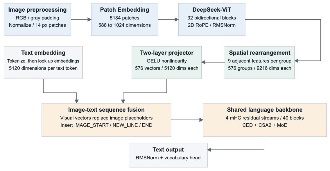
The above figure takes a 1008 x 1008 pixel square image after preprocessing and padding as an example:
| Stage | Operation | Example shape | Description |
|---|---|---|---|
| Image preprocessing | RGB, size planning, resize/pad, normalization | Preserve 2D layout | |
| Split into patches | Non-overlapping blocks | Grid is | |
| Patch embedding | Linear projection after flattening | Each patch independently uses the same set of weights | |
| DeepSeek-ViT | 32-layer bidirectional vision Transformer | Retain all patch positions, no CLS aggregation path | |
| Spatial rearrangement | non-overlapping grouping | Grid changes from to | |
| Two-layer projector | Linear, GELU, Linear | The intermediate layer is also -dimensional | |
| Image span assembly | Insert row separators and start/end markers | Contains positions | |
| Image-text fusion | Interleave with text embedding in original order | includes text and all image spans | |
| mHC expansion | Establish 4 residual streams | Each position enters the shared language backbone | |
| Language backbone | 40 layers CED/CSA2/MoE | Hidden state dimension remains unchanged | Finally outputs text through the vocabulary head |
Image preprocessing: It should be noted that it does not perform text recognition like OCR. After the file is loaded, it is directly decoded via load_image and converted to RGB. Then it checks the minimum pixel area. If the original image area is below , it scales up the target size proportionally. Subsequently, it aligns the two edges upward to a multiple of vision_patch_size=14, and fills the aligned blank areas with RGB gray. And note that it checks whether the expanded image span exceeds the vision_max_n_token=1024 budget. When exceeding the budget, it re-computes a smaller target canvas based on the aspect ratio.
Let the pixel size after preprocessing be , the patch side length be , and the spatial merge factor be . The code first makes the pixel side length an integer multiple of :
The Aligner allows the patch grid to not be divisible by 3, because it pads zeros on the right and bottom of the feature grid:
The merged visual grid and its content token count are:
And what the local preprocessing function actually budgets is:
Among them, one IMAGE_NEW_LINE per row, plus IMAGE_START and IMAGE_END.
For the paper's "supporting input resolutions up to approximately 1344 ×1344 pixels", it is essentially constrained by vision_max_n_token=1024. For example, according to the paper's , , and then the token count after subsequent downsampling is 1024, but considering that adding tags within the span will exceed the vision_max_n_token=1024 budget, this image will be scaled to , i.e., tokens, plus 31 NL tags and 2 START/END tags, for a total of 994 tokens.
And common screen resolutions such as will be scaled to , for a total of 968 tokens.
Then the image is normalized according to the RGB channels as:
Continuing with the image as an example, the code then splits the image into non-overlapping blocks. If the row-column coordinates of an image block are , and the intra-block coordinates are , the value it takes out is . It first traverses the columns within a row, then enters the next row, obtaining image blocks with shape . Splitting into blocks rewrites the spatial coordinates as block numbers and intra-block coordinates.
Patch Embedding: All numbers of each block, then flatten each block, and all blocks share the same linear layer with bias. Finally, a matrix is obtained. Note that the paper explains why the convolution needs to be replaced by linear projection, the main reason being to ensure compatibility with the Muon optimizer.
DeepSeek-ViT: Next, 32 layers of ViT processing are performed to give them intra-image context. Both the input and final output are . Each layer first performs RMSNorm on the current features, then computes attention and adds back the residual; subsequently normalizes again, executes the SwiGLU feed-forward network, and adds back the residual. After the 32 layers, there is one more RMSNorm at the end of the vision tower.
Taking the attention of one of the layers as an example, a linear layer first generates Q, K, V from the normalized features, with a total output width of . The three are respectively organized into , that is, 16 heads, each head 64-dimensional. Before computing scores, 2D RoPE rotates Q and K according to the original row-column coordinates, and does not rotate V. Attention solves cross-position communication, while the subsequent SwiGLU mainly does channel transformation within each position. It first projects to dimensions and splits into two branches, applies SiLU to the gating branch, multiplies it element-wise with the other branch, and then projects back to 1024 dimensions. In this way, one layer simultaneously contains two kinds of processing: "fetching information from other positions" and "reorganizing features at the local position".
Spatial rearrangement: It loads 9 adjacent features into the same wide vector, and adopts downsampling. The specific approach is as follows:
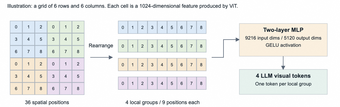
2-Layer MLP: Used to generate tokens for the LLM, aligning hidden_dim = 5120.
Finally, within the token span generated by the image, some markers still need to be supplemented, as shown in the figure below:
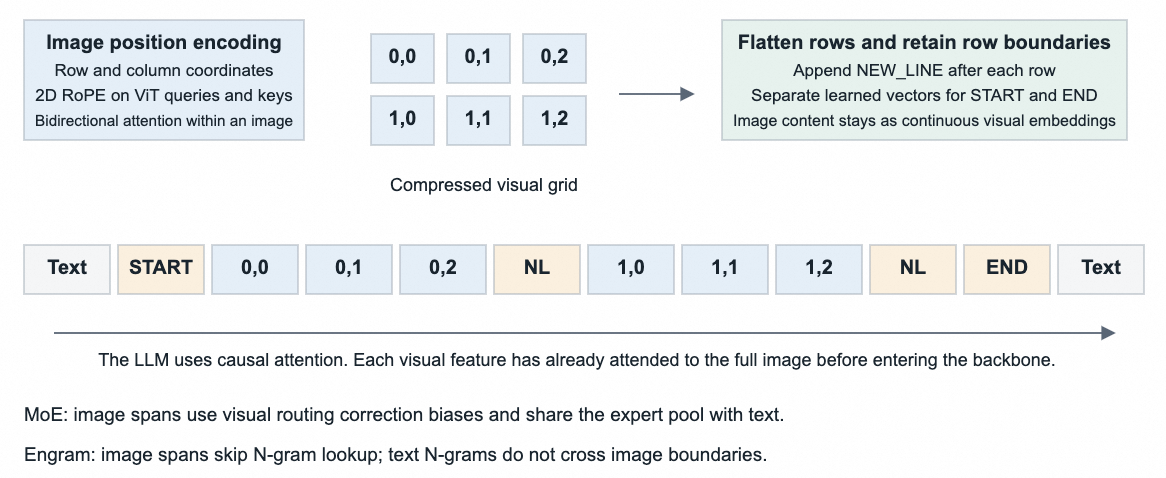
Then these tokens will be sent to the backbone network. Here there is another optimization, multimodal auxiliary-loss-free load balancing for MoE. Image and text tokens exhibit different representation distributions, and may form different expert routing preferences in MoE. Therefore, balancing their aggregated load may mask the imbalance within each modality. To solve this problem, the DeepSeek team maintains a set of per-expert correction biases for text and image tokens respectively. During routing, each token uses the correction bias corresponding to its modality for expert selection, while retaining the original routing score to weight the output of the selected experts. After each training step ends, these two sets of biases are independently updated according to their respective expert loads. This design balances expert usage within each modality, helping stable and efficient multimodal training.
2.2 Causal Encoder-Decoder(CED)
2.2.1 Why is CED needed?
The substantive problem is that in Agent workflows, frequent tool calls will generate a large number of prefill requests, which causes heavy computation overhead when the KV Cache misses.
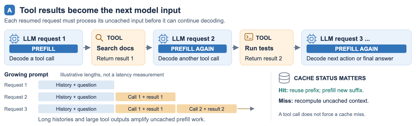
To alleviate this prefill bottleneck, the authors propose a Causal Encoder-Decoder (CED) architecture inspired by YoCo 《You Only Cache Once:Decoder-Decoder Architectures for Language Models》[2]. YoCo reduces prefill computation by letting the upper-half layers directly share the KV Cache produced by the lower-half layers.
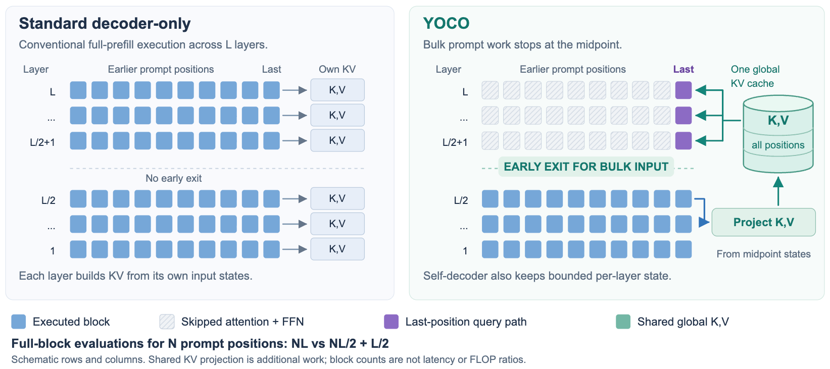
In terms of concrete implementation, YoCo separates the production and consumption of historical memory: the lower half establishes memory, and the upper half repeatedly reads memory, but no longer generates the per-layer historical KV that must be saved for subsequent inference.
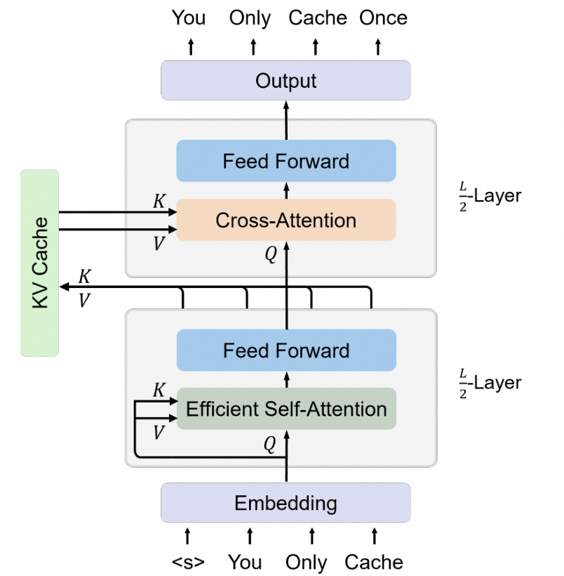
Here let us briefly expand on the entire architecture evolution process of YoCo. First, the attention mechanism of each layer of a Decoder-Only model causes each layer to have KV computation during Prefill, which is the root cause of low efficiency.
The first intermediate solution is to use the SWA algorithm, which through a fixed sliding window, each layer produces KV, that is, the Efficient Self-Attn (ESA) mentioned in YoCo's original paper. But if all layers use SWA, the global attention mechanism will be lost (note: in the original paper, ESA can optionally be SWA or gRet...). Another solution is to split the entire model in depth, with the first half using ESA to produce global KV, and the second half using standard Attention to read the first half's KV, so that the global attention mechanism can be restored. But we need to determine which layer the second half's KV comes from?
The final determined solution is that the second half's KV is projected from the -th layer's hidden state via , which constitutes the YoCo architecture.
In fact, YoCo's solution has been tried by some base model teams, usually described with a different name called KV-Mirror. Some teams have not made it public. The publicly searchable one is Tencent's WeLM 《Building Effective Sparse MoE Models with Moderate Resources》[3].
2.2.2 Concrete implementation of CED
On top of the YoCo concept, CED introduces a series of structural improvements, simultaneously increasing the overall capacity of the KV Cache and the computation depth of KV generation, finally successfully reducing prefill computation by nearly half while maintaining performance comparable to the baseline.
For global attention, CED regards the bottom layers of the Transformer as a Causal Encoder. For the upper-half layers (i.e., the Decoder, ), the KV entries are no longer derived from their respective hidden states , but are directly projected from the -th layer's hidden state via layer-dependent projection weights ( and ):
Where and represent the KV entries and the corresponding compression weights respectively. This design allows CED to obtain the global KV Cache of the upper layers at an extremely low computational cost, only needing to compute the first half of the layers during the prefill stage.
Specifically, CED divides the model into two parts, Causal-Encoder and Decoder, with 20 layers each. By comparison, YoCo names the two parts Self-Decoder and Cross-Decoder, mainly distinguishing the two parts by the information source of attention. The first half processes the sequence through efficient self-attention, and the second half uses the queries produced by its own layers to read the shared KV generated by the first half. DeepSeek changed to a different observation angle: since the key responsibility of the first half is to generate reusable context representations, it can be seen as an Encoder; the upper half uses these representations to continue computing predictions, so it is called a Decoder. In YoCo's paper viewpoint, it mainly emphasizes that the Self-Decoder is about "how to efficiently process sequences", and the Causal Encoder emphasizes "what it provides for subsequent networks". The distinction between the Encoder/Decoder names is only a difference in perspective.
In YoCo, the first half adopts ESA (gRet or SWA), while in CED, the first two layers of the Causal-Encoder are also SWA, and the subsequent 18 layers adopt CSA2, which is a Sparse Attention with compression combined with SWA. It calls the KV built by Sparse Attention Global KV, and calls the KV built by SWA Local KV, which are concatenated and then used with Q to compute the Attn-Score. We will expand on this in detail in a later section and elaborate on the CED architecture in combination with CSA2.
For SWA, CED maintains regular per-layer computation in all layers: the local KV of any layer is directly derived from the current layer's hidden state , which actually increases the computation depth of local KV generation. But maintaining per-layer computation requires an SWA replay process: computing the SWA KV Cache for the Decoder during the prefill stage requires additional processing of tokens ( is the window size). For multi-turn interactions where each turn's prompt is relatively short, this part of the Decoder overhead cannot be ignored. Fortunately, prior work (Chen et al., 2025) shows that the actual effective receptive field of SWA is far smaller than the theoretical value . Inspired by this observation, the authors introduce Decoder SWA Bounded Replay: only compute the SWA of the last tokens of the prefill prompt for the Decoder, thereby significantly reducing the computation cost.
1. Why does SWA actually increase the computation depth of local KV generation?
First denote the Encoder depth as , the Decoder depth as , and the window size as . CED's global KV comes from the Encoder boundary representation:
Although the first half has many layers, the global memory read by the Decoder still comes from the projection of . Subsequent layers can produce different queries, but this will not turn the source of the historical global KV into a deeper-layer representation. And each subsequent layer adds SWA-based local KV, which retains the path of "each layer generates KV from its own input representation". "Depth increase" refers to: the KV of these recent positions can contain deeper-layer computation results, not just different projections of the same Encoder boundary representation.
2. Why is Bounded Replay needed?
But these Local KVs also bring some problems. For ordinary complete prefill, there is no such problem: all prompt words pass through all layers, and the local KV of each layer is naturally generated with the forward computation.
But CED wants most historical positions to stop computing after the Encoder ends. At this point, although the global KV can already be prepared, these historical positions have not passed through the Decoder, so the Local KV of the deep Decoder layers has not yet been generated. Decoder SWA Bounded Replay is to make up for the Decoder Local KV missing after CED ends prefill early, while avoiding the cost of restoring these KVs offsetting the benefit of early exit.
Since SWA only saves the local KV of the most recent positions, it seems that replaying the last positions is enough. But the problem is: the representations of these positions in the deep layers still depend on earlier positions outside the window. For example, each layer window is 4. To compute the second-layer representation of position 100, the representations of first-layer positions 97 to 100 are needed. And first-layer position 97 needs to read input positions 94 to 97. Therefore, the deeper the recovery, the more it needs to trace back forward. For a -layer Decoder, the historical span for exact recovery is approximately:
If each tool call only adds a few dozen words, but to restore the cache, thousands () of historical positions must pass through the Decoder, the computation saved by early exit of prefill may be consumed by a large amount of replay. The authors referred to the work of 《PowerAttention: Exponentially Scaling of Receptive Fields for Effective Sparse Attention》[4]. This is a paper studying the receptive field of sparse attention and cross-layer information propagation. In its Section 4.3 there is an experiment that evaluated the model on a passkey retrieval task. In its SWA experiment with about a 2K window, the authors estimated that information has decayed quite weakly after propagating through about 6 layers.
Therefore DeepSeek adopts the Bounded Replay approach, and the role of Bounded is to limit this overhead: only replay the last positions, no longer continuously tracing back forward for exact recovery. The cost is that the reconstructed Local KV is in an approximate state. The beginning of the replay segment lacks earlier local dependencies, and subsequent deep-layer representations may change accordingly.
However, we note that in CSA2 what is truncated is the reconstruction range of the Local SWA state, not the global memory. When replaying the last positions, the Decoder can still read the Global KV of longer history according to the causal and sparse attention rules. Therefore, DeepSeek accepts this approximation and controls the impact through quality evaluation and post-training adaptation.
3. Why is this problem important?
Under long prompts, tail replay is just a small piece of work outside the Encoder's large-scale computation. But in Agent multi-turn interactions, most of the history may have already hit the global cache, and the truly newly added content in this turn is very short. Let the newly added length of this turn be . The Encoder main body work of the new content roughly grows with , but the cost of restoring the Decoder local state does not automatically shrink with . For example, when , , the historical span of exact recovery is about positions. Even if only a few dozen positions are newly added in this turn, it may still look back at a very long tail to restore the local state, and then execute multi-layer computation.
Bounded replay limits this restoration work to the most recent positions passing through the Decoder, limiting the state restoration of each turn to a fixed overhead.
Overall, for sequence length , CED reduces the prefill complexity from to , actually halving the total computation.
Why is the computation halved?
For the cold-start prefill of a long prompt, the Encoder processes all positions: , and the Decoder only processes tail positions:
So the main body workload is:
Substituting , and comparing with the full computation :
When , the second term is very small, and the ratio approaches . Taking DeepSeek V4.1 Flash's , as an example, assume the prompt length is . The full computation is about token-layers; CED's Encoder plus bounded replay is about , which is of the former.
2.3 CSA2
2.3.1 Why is CSA2 needed?
Serving long contexts requires simultaneously controlling KV cache storage and attention computation. These costs can be reduced along three dimensions with a multiplicative relationship:
Entry size dimension: For example, GQA reduces the number of KV heads, and MLA shares a small latent representation across different heads Sequence dimension: where every tokens are compressed into one entry, such as CSA and HCA in DeepSeek-V4; Layer dimension: where certain layers reuse the cache and selection results of other layers, instead of retaining their own cache and selection results, or are entirely replaced by more efficient layers.
In the work on the layer dimension:
《Reducing Transformer Key-Value Cache Size with Cross-Layer Attention》[5] proposes cross-layer attention, letting a portion of attention layers directly read the KV produced by earlier layers, thereby avoiding saving an independent KV cache per layer. 《IndexCache: Accelerating Sparse Attention via Cross-Layer Index Reuse》[6] reuses Top-K indices across layers to reduce Indexer computation 《You Only Index Once: Cross-Layer Sparse Attention with Shared Routing》[7] computes sparse routing only once and shares it with all layers 《HySparse: A Hybrid Sparse Attention Architecture with Oracle Token Selection and KV Cache Sharing》[8] lets sparse layers reuse the KV cache of dense layers.
However, merely reusing indices does not save the main KV storage, sharing routing across the entire network limits performance, and hybrid designs still retain full attention layers; more importantly, none of these methods cover all three dimensions with a multiplicative relationship.
Analyzing carefully, although Cross-Layer Attention (CLA) can share KV across layers and reduce independent KV copies, each layer still computes its own attention; KV storage is saved but computation is not; IndexCache shares Top-K indices between some layers, which can reduce the number of Indexer runs, but the main KV is still saved per layer, so although some Indexer computation is saved, storage is not. And YOIO reuses the Decoder-Decoder structure of YOCO, saving half of the KVCache, but multiple layers of Sparse Attention in the cross-decoder need to share one set of selected TopK candidate set, which has an impact on the model's performance. HySparse uses Full Attention to produce KV, and although sparse layers can reuse these KVs, the efficiency of the full Attention computation will still affect performance.
Before introducing CSA2, we can review in detail DeepSeek's optimizations of Attention computation over the past few years. In MLA, joint low-rank compression is done on the K/V representations of all heads, compressing on the entry size dimension. Then Sparse Attention (DSA) was introduced in DeepSeek V3.2, reducing the computation demand of Attention. Then in DeepSeek-V4, compression on the sequence dimension was added through CSA (compression ratio 4:1) and HCA (compression ratio 128:1). And CSA2 further pushes compression toward the layer dimension.
CSA2 jointly utilizes these three dimensions: it shares the main KV and Indexer K across layers, and allows layers to reuse Top-K indices, while decoupling cache sharing and index reuse. It combines these reuse strategies with a simplified compressor and a hierarchical sparse Indexer, the latter of which narrows the search range of subsequent index layers in the Decoder.
Some subtle computational differences from CSA: Similar to CSA, CSA2 includes a lightweight Indexer that uses Indexer Q and Indexer K to score the main KV entries, selecting Top-K entries for each query, and each Q simultaneously attends to the selected entries and the intra-layer local sliding window KV (SWA KV).
The Compressor of CSA2 also has some differences. First, it includes the special case of compression ratio 1, that is, the ability not to compress the Main KV, used for Decoder Layers.
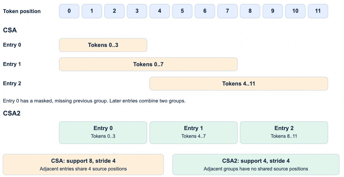
In the concrete implementation, the Causal-Encoder uses a compression ratio of which can reduce the number of entries and index candidates of each copy of the Main KV; the Decoder uses to retain per-token addressability. After combining with CED and cross-layer cache sharing, the Decoder does not need to save an independent long-sequence main KV for each layer, so it can allocate a portion of the space budget to a finer sequence granularity.
At the same time, CSA2 simplifies the Compressor and Indexer. In CSA, a compression ratio means that each main KV entry is produced by original KV cache entries, and there is overlap between the source entries used by adjacent compressed entries. It also includes absolute position embeddings to encode the positions of these entries during compression. CSA2 removes this overlap and the absolute position embeddings.
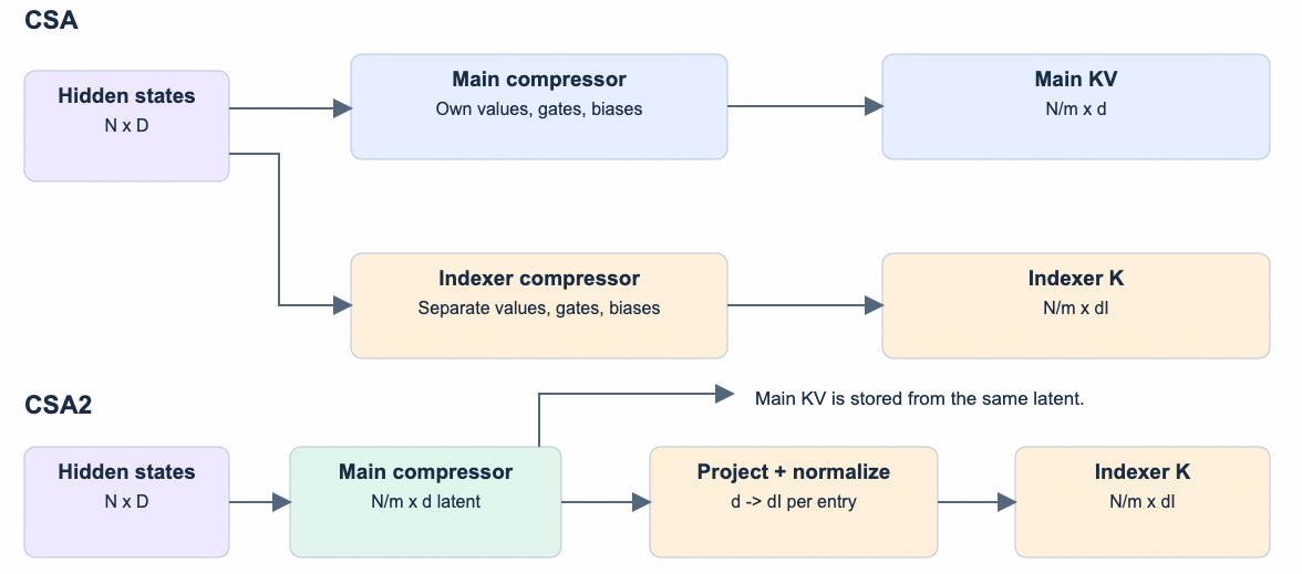
In addition, CSA2 obtains the Indexer K by projecting the main KV entries, replacing CSA's independent compression path starting from the hidden state. Both of these designs simplify the implementation and improve training efficiency.
2.3.2 Cross-layer KV and Index reuse
Specifically, CSA2 mainly adds data reuse in the layer dimension on the basis of CSA. From the perspective of computer architecture, we can regard the Attention block as a compute component, MoE/FFN as a storage component, and the KV-related part as the Cache of computation. From this perspective, we can regard the cross-layer reuse of KV and Index as a kind of Data Locality processing, as shown in the figure below:
Cross-layer reuse is mainly divided into three modes, as shown in the figure below:
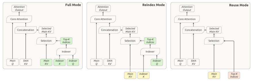
The difference between these modes lies in how the Main KV, Indexer K, and Top-K Indices are obtained. Green squares indicate quantities computed at the current layer; yellow squares indicate the main KV and Indexer K reused from the most recent Full mode layer; red squares indicate the Top-K indices reused from the most recent layer that generated indices. In addition, all three modes compute Main Q and SWA KV at the current layer.
Full mode This layer computes its own Main KV and Indexer Q, obtains the Indexer K by projecting from the Main KV, and runs the Indexer, producing new Top-K indices. Therefore, it executes the complete CSA2 computation path, and the responsibilities borne by each component are the same as those of a complete CSA layer in DeepSeek-V4.
Reindex mode This layer reuses the most recently available Main KV from a previous layer, as well as the corresponding Indexer K. And it computes its own Indexer Q, re-scores the reused Keys, and generates new Top-K indices. This allows the sparse selection to vary across layers, while the Main KV and Indexer K remain shared.
Reuse mode. This layer reuses the most recently available Main KV, as well as the latest Top-K indices computed for that Main KV by a previous Full mode layer or Reindex mode layer. It uses this selection to execute the attention computation, does not compute Indexer Q, and does not evaluate index scores.
Sharing the Main KV and Indexer K reduces the storage footprint of the KVCache, while reusing the Top-K Indices can avoid additional Indexer computation. The Reindex mode allows the selected entries to vary across layers while retaining cache sharing. We will analyze the specific mode usage in combination with CED.
2.3.3 The combination of CED and CSA2
In the Causal-Encoder, we can regard it as a structure composed of the following macro blocks. First is a 2-layer standard SWA block, then followed by a structure composed of three macro Encoder blocks. Engram is injected before the second SWA block and the last Encoder block, as shown in the figure below:
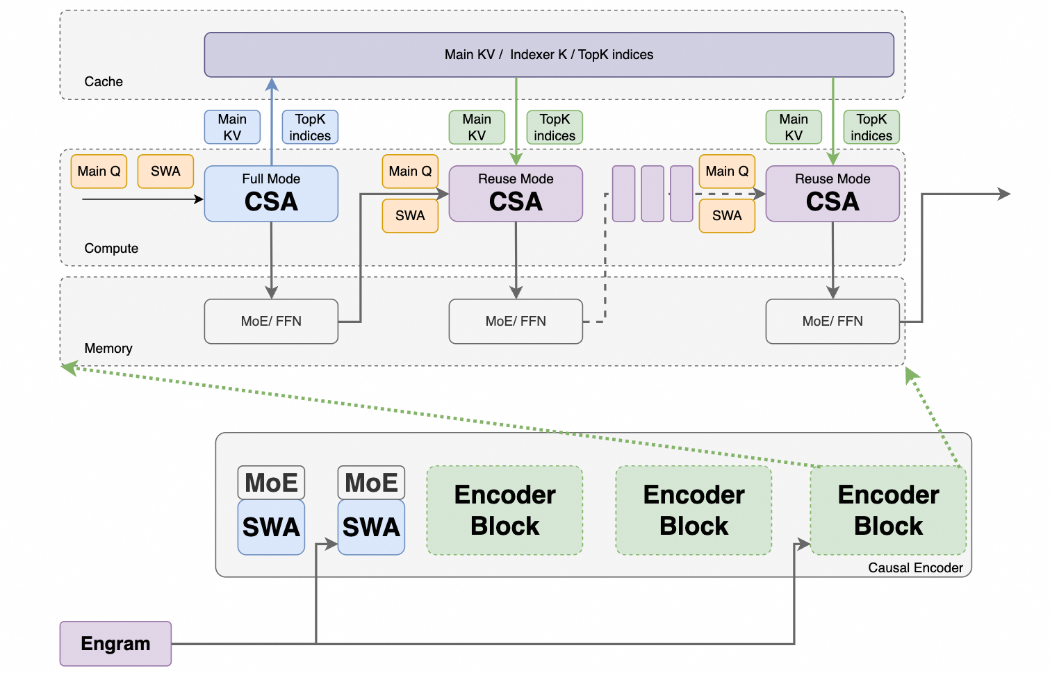
An Encoder block is a 6-layer structure, with the first layer being a Full mode CSA2, and the subsequent 5 layers being Reuse mode CSA2. The above approach can better describe the entire cross-layer reuse mechanism.
1. Why regard 1 layer Full + 5 layers Reuse as an integral Encoder block?
The first-layer Full mode CSA2 will compute and write the entire Main KV and TopK indices. The subsequent 5 layers of Reuse mode CSA2 will all reuse the Main KV and TopK indices produced by the first layer. In short, both KV and TopK selection are reused in the Reuse mode block, and what each layer actually modifies is Q.
Therefore, for the entire Encoder block structure containing 6 layers, we can regard it as a recursive Transformer structure that performs recursion by modifying Q at each layer.
2. What is the role of the first two layers SWA + Engram?
Described in one sentence: the first layer provides local context, Engram injects memory addressed by short patterns and controlled by context, and the second layer integrates the two into a representation usable for subsequent compression.
The first-layer SWA window size is , and the set of positions that position can read is:
For example, the same word in different sentences will assign different weights to different nearby positions. The output of the first layer is transformed by SWA into a representation processed by local context. Then comes the injection of Engram. Regarding Engram, there is a detailed analysis in the previous article 《On DeepSeek Engram: Conditional Memory》.
Engram reads the 2-gram, 3-gram, and 4-gram ending at the current position, then concatenates after hash table lookup. Therefore, Engram has the ability to encode repeatedly occurring phrase patterns, local combination regularities, etc. into the parameter table. And the output of the first-layer SWA provides context gating for Engram. Note that, compared to directly injecting Engram at the first layer, the output after first-layer SWA processing is already a representation that combines local context.
Engram's injection directly does a residual update of the current position; it does not directly write the current position's memory into other positions. But the second-layer SWA can read the Engram-enhanced representation of each position in the window. Therefore, both the Q and local KV of the second-layer SWA can be influenced by Engram to enhance relevant phrase patterns, local combination regularities, and other information. After the second-layer SWA processing, the integration of local information is completed. Therefore, the first two layers form the following order:
On the other hand, the result of the two layers of SWA expands the receptive field length to: . Therefore, in the CSA2 processing starting from the third layer, the input contains: token embedding / the result of the two layers of local context computation / the Engram memory injected after context gating and integrated—these processed local representations. This is also one reason why the Compressor in CSA2 does not need to perform Overlap processing.
Then let us look at the structure of the Decoder. We can similarly regard it as a structure composed of 5 Decoder Blocks:
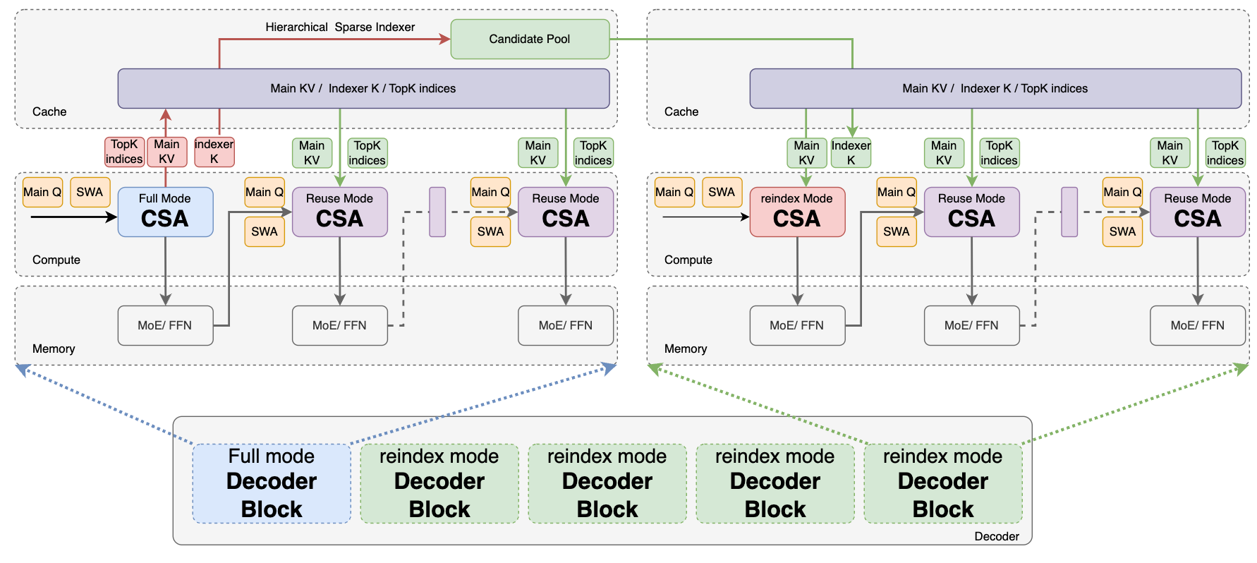
Among them, the first CSA2 in the first Decoder Block is Full Mode, so we also call it the Full Mode Decoder Block. Similarly, the subsequent 4 Decoder Blocks are also called Reindex Mode Decoder Blocks. Note that all CSA2 in the Decoder have a compression ratio of 1, and only Reindex Mode CSA2 is used in the Decoder.
The first layer of the Full Mode Decoder Block is a Full Mode CSA2. Like the Full Mode CSA2 in the Causal-Encoder, it computes its own Main KV as well as Indexer K and TopK indices. The Main KV and TopK indices will be reused by the subsequent 3 layers of Reuse Mode CSA2. But it introduces a Hierarchical Sparse Indexer (HSI) processing approach, constructing a block-level selection as the Candidate Pool for the subsequent Reindex Mode CSA2 through the scores when computing the Top-K Indices. We will expand on this in detail in a later section.
Reindex Mode Decoder Block: In the Decoder, there are 4 Reindex Mode Decoder Blocks after the Full Mode Decoder Block. Its internal first layer is a Reindex Mode CSA2. The Reindex Mode CSA2 will recompute its own Indexer Q for scoring, and select its own Top-K entries within the Candidate Pool.
2.3.4. Hierarchical Sparse Indexer (HSI)
Cross-layer index reuse reduces the number of Indexer evaluations, but the remaining Indexers still need to score all causally visible context. For ultra-long contexts, this cost is still a major computational bottleneck.
In 《HISA: Efficient Hierarchical Indexing for Fine-Grained Sparse Attention》[9], it studies how to use "block-level coarse filtering + token-level fine filtering" to reduce the overhead of the sparse attention indexer.
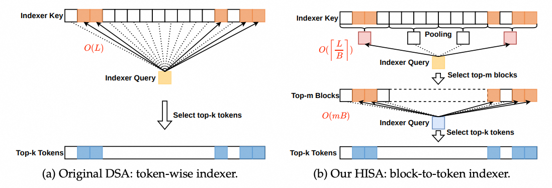
As shown in the figure, it divides the prefix into blocks of size about by consecutive positions, with the -th block being . The number of blocks is . Each block maintains the Indexer's mean:
The mean serves as an auxiliary function for searching. The original token Indexer and Main KV are still retained. During decoding, the vector sum and count can be maintained for the current block, a new token only updates one block, and the completed historical blocks reuse the summary.
The first stage reuses the same set of to score the block means:
Only the high-scoring blocks are retained, then expanded into a candidate position set:
The second stage computes the original for , and selects the final positions from the candidates:
The DeepSeek team found that in the Decoder, the information of the shallow-layer Indexer can naturally be used to limit the candidates considered by the deep-layer Indexer, without needing to add any extra state. Therefore the authors introduce the Hierarchical Sparse Indexer (HSI), used only in the CED decoder, to reduce repeated scoring during decode. For each query, the first Full Mode layer constructs a Candidate Pool as the search domain for the subsequent Reindex Mode layers. When the Candidate Pool size is fixed, the per-query cost of the deep-layer Indexer changes from growing linearly with the context to a constant. This mechanism is training-aware, introduced in the post-training stage: training and inference impose exactly the same candidate restriction, so that the deep-layer Indexer is optimized under the search domain used for inference.
The working principle of HSI is as follows:
The first Full Mode CSA2 scores all causally visible main KV positions, producing Top-K indices for its own attention; at the same time it performs block-level candidate selection: each block takes the maximum index score of its internal positions, selects the several blocks with the highest scores, and collects the positions covered by these blocks into a candidate pool larger than the final Top-K set. For example, select 2048 blocks, each block with 8 positions, obtaining 16384 candidate positions. The candidate pool decides "where to search" for the subsequent Indexer, and the final Top-K decides "which entries to read" for each layer.
The subsequent Reindex mode layers only score the candidate positions of the corresponding query, and select their own Top-K entries within the pool; the Reuse mode layers do no new indexing and directly use the latest Top-K indices computed for the reused main KV. Thus the candidate pool is shared across index layers, while the final selection can differ.
When the candidate pool size is fixed, the number of positions scored per query by each subsequent Indexer is independent of the context length and bounded; the first Full mode layer still needs to scan the entire causally visible range. Therefore hierarchical indexing reduces the cost of subsequent Indexer evaluation while retaining the initial full-range scan.
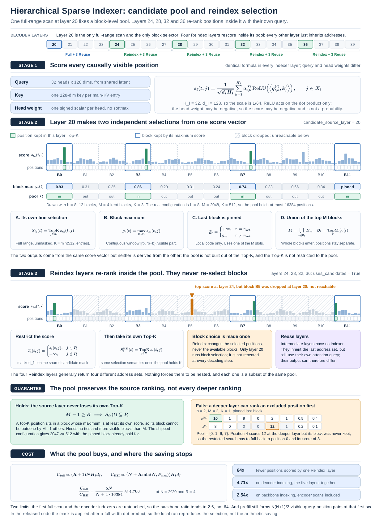
The difference from HISA is that HISA needs to first perform block pooling scoring at each layer, then perform sparse TopK selection. And HSI takes the block maximum value from the complete position scores already obtained at the shallow layer, subsequent layers share the candidate range, and adapt to the restriction in post-training. Both do coarse filtering first then fine selection, but the basis for coarse filtering is different.
In addition, HSI taking the block maximum value avoids the peak dilution that mean pooling may cause.
1. How does the Full Mode layer generate the Candidate Pool? The candidate block width candidate_block_size is , the upper limit of the number of blocks candidate_topk_blocks is , and the final selected TopK is . Use to denote the -th causally visible block,
The first layer first computes the complete Indexer Score . For itself to produce TopK indices
The same set of scores is also used for block maximum reduction,
The corresponding implementation is scores = F.pad(logits, (0, -width % block_size), value=-torch.inf) padding the last block with , then unflatten splits the history axis into the number of blocks and 8 positions per block, and amax(dim=-1) exactly implements . Finally, at most blocks are selected by block score
In addition, a boundary strategy is added. It temporarily sets the block score containing the latest visible position to , forcing this block to occupy a selected-block quota. That is
For the selected blocks, a bitmap is produced, then through repeat_interleave(block_size, dim=-1)[..., :width] the block flags are expanded into a bitmap of the same width as the original scores, constituting the candidate pool used for the subsequent reindex mode computation.
In addition, we also need to note that the paper states "This mechanism is training-aware, introduced in the post-training stage: training and inference impose exactly the same candidate restriction, so that the deep-layer Indexer is optimized under the search domain used for inference." But the specific post-training method is not disclosed here.
Assuming HSI is not used, each layer of the Decoder that needs to re-index can search the complete history for the most relevant 512 positions. After using HSI, the first retriever first shrinks the history into a list containing at most 16384 positions, and the subsequent retrievers can only each pick 512 positions from the list. If during training the subsequent layers are still allowed to search the entire history, but when deployed online they are suddenly only given a list, there will be an inconsistency between the training-inference distribution and selection, affecting performance.
The paper states that DeepSeek-V4.1-Flash already uses sparse attention from scratch in the pre-training stage, first training with 64K sequences, then extending to 1M, and clearly states that HSI is introduced in the post-training stage. That is to say, the pre-training stage should have no HSI on the model structure. The Reindex Mode layers still use complete computation. In the post-training stage, to make the exclusive parameters of the deep-layer Indexer truly learn, there must also exist an Indexer loss or other gradient estimation mechanism, but the report does not disclose the loss form. We speculate that it uses a hybrid loss function:
Among them, makes the backbone adapt on the restricted candidate set; may use the main attention distribution to distill the Indexer's continuous scores. Combined with the implementation of DSA, we speculate it to be:
Where denotes stop gradient, is the set of queries with valid supervision at this layer, and is the explicitly specified supervision support set. is the auxiliary objective coefficient.
2.4 Efficient architecture extensions
2.4.1 Single-Pass mHC
Regarding mHC, there is a detailed analysis in the previous article 《On DeepSeek mHC》. It maintains residual streams between adjacent Transformer blocks, as shown in the figure below
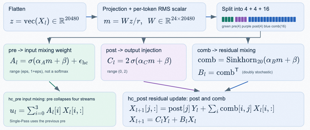
For each token, use to denote these streams, where is the block index and is the hidden dimension. These streams are updated as follows:
Where , and are per-token coefficients predicted from . The coefficient predictor includes normalization and projection. But there is a data dependency during computation. Single-Pass mHC shifts the input mixing coefficients by one block, that is, each block uses the mixing coefficients produced by the previous block, thereby eliminating the dependency:
The comparison is shown in the figure:
2.4.2 Engram
Regarding Engram, there is a detailed analysis in the previous article 《On DeepSeek Engram: Conditional Memory》. The differences between DeepSeek-V4.1-Flash and the original paper's model structure are as follows: the n-gram is extended to {2,3,4} and the short causal convolution is omitted, because of its trade-off between the complexity of the inference software stack and the performance gain. In addition, momentum-based updates are used, followed by Sinkhorn Balance to optimize the Engram Embedding.
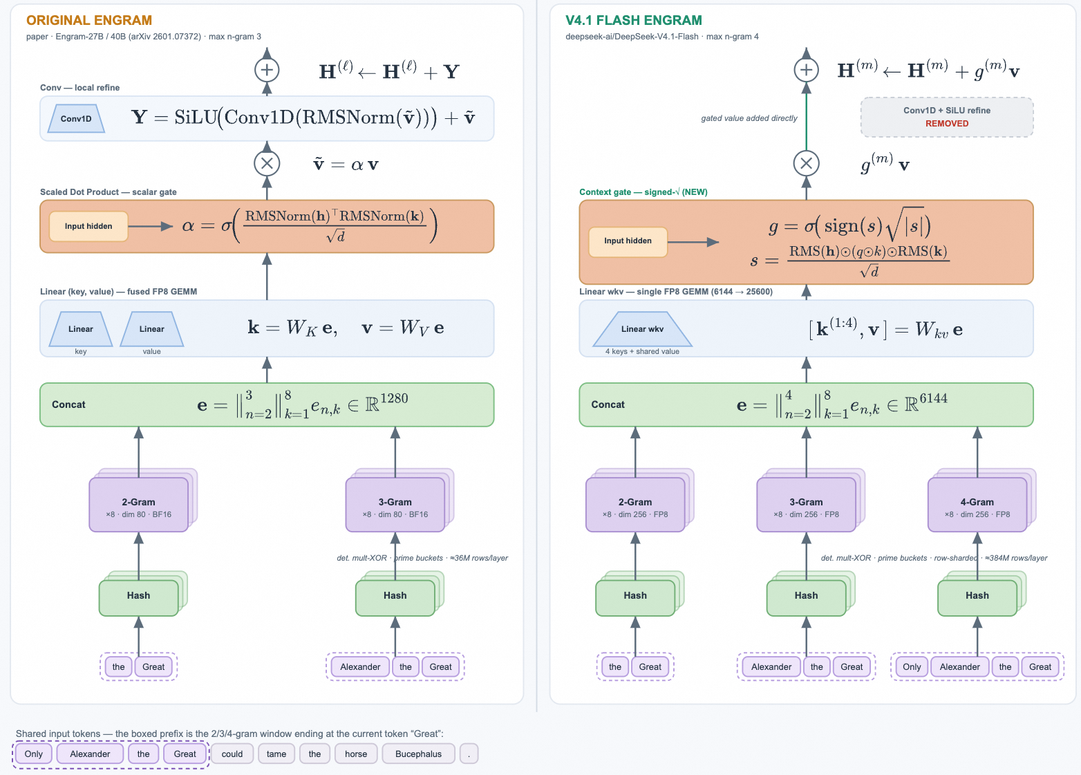
It evenly distributes the 196B Engram parameters to two modules. Each module adopts N-gram orders , each order contains 8 hash heads, and the total embedding dimension is 2048. Each head indexes a table with about 16M entries, and each table size is chosen as a distinct prime number. Both the embedding tables and the key/value projections use FP8 precision. The modules are placed at layer 1 and layer 14, that is, before the Full mode CSA2 in the second SWA and the last Encoder Block, to balance memory usage between training pipeline stages.
During inference, deterministic addressing allows prefetching embeddings from host memory via background RDMA transfers, and the prefetching of the first module overlaps with the computation of the first Transformer block.
2.4.3 DSpark
Regarding Dspark, there is already a detailed analysis in the previous article 《A Detailed Discussion on the Principle of DSpark Speculative Decoding》.
In DeepSeek-V4.1-Flash, the Draft Model consists of three Transformer blocks, whose sliding attention window is 128 tokens. One forward computation will compute in parallel the basic unnormalized scores of five draft positions, while a lightweight Markov head models the dependency between Draft tokens.
DSpark is introduced in a dedicated stage after pre-training. In this stage only DSpark is trained, while keeping the backbone frozen. During post-training, DSpark continues to be trained together with the backbone, but the gradient of the DSpark objective is not propagated to the backbone. This keeps DSpark aligned with the continuously evolving policy, thereby both accelerating online inference serving and accelerating the trajectory generation of reinforcement learning RL and on-policy distillation OPD.
2.4.4 FP4 Main KV Cache
Further reducing the storage footprint of the KVCache from the numerical precision aspect. In DeepSeek-V4, quantization-aware training QAT was already used for the FP4 Indexer Q and K to accelerate index computation and shrink the indexer cache. Here it is mainly about FP4 processing for the Main KV. To support as many hardware platforms as possible, the OCP standard MXFP4 format is still adopted. Here the role of FP4 is to reduce storage, not to accelerate matrix multiplication. Before the attention computation, the cache values are dequantized to a more accurate format, without needing native support for matrix multiplication in this format, thereby maintaining compatibility across hardware platforms.
The figure below shows NVFP4(E2M1) as a reference:
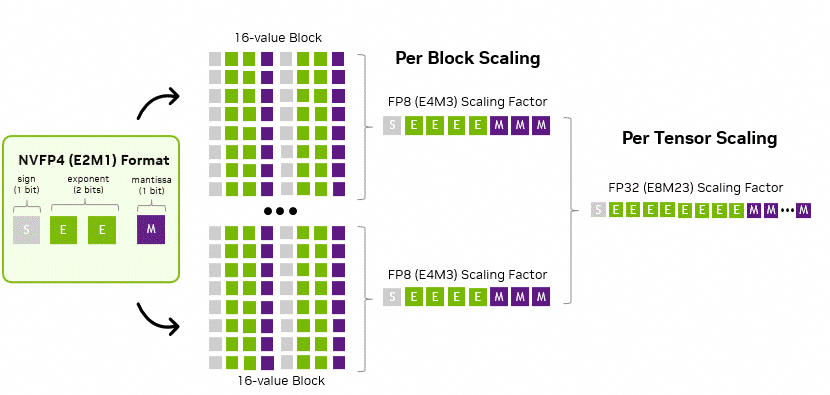
DeepSeek chooses E2M1, with every 16 channels sharing one E4M3 scale factor, following NVFP4, but omitting its second-level global scale factor, to balance precision and simplicity. As shown in the figure below:
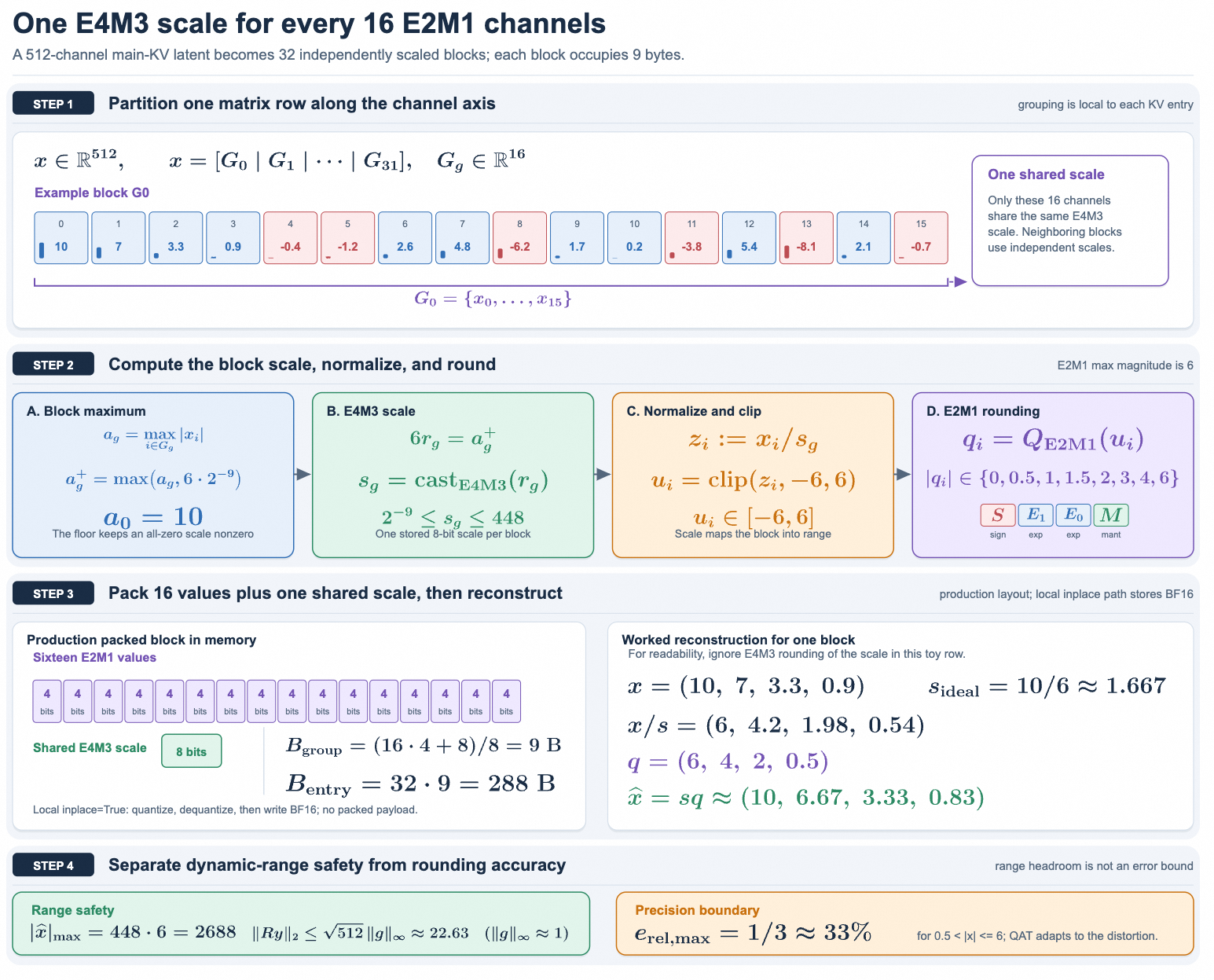
After omitting this scale factor, the main KV cache still has ample dynamic range: this format supports a maximum magnitude of , far higher than the upper bound of the cache magnitude. In DeepSeek-V4.1-Flash, the maximum RMSNorm weight magnitude obtained by training is about 1. After RMS normalization, the L2 norm of the 512-channel KV latent variable is at most about . RoPE preserves this norm, so the maximum absolute value of each channel after rotation is also bounded by about . In addition, the maximum magnitude observed during training is about 10. Therefore, omitting the global scale factor causes no measurable precision degradation and simplifies the cache layout.
To support FP4 main KV cache storage in DeepSeek-V4.1-Flash, QAT is introduced during post-training. The non-RoPE component and the RoPE component use the same quantization format. In addition, the cache is quantized after RoPE: in experiments, quantizing before RoPE only brings a slight precision improvement, but introduces additional overhead during decoding. Since the KV cache of sliding window attention SWA is sensitive to quantization, FP8 precision is retained. Compared with the FP8 Main KV cache of DeepSeek-V4, this format makes the storage footprint in HBM and when offloaded to SSD both nearly halved.
3. Why can KV be saved?
First, we will count the sources of KV Cache savings in the first section. Overall, the optimization of KVCache by DeepSeek-V4.1 Flash is divided into several parts. First, FP4 Main KV saves half of the overhead, CED reduces a large amount of computation consumption during Prefill, and the most critical is still the cross-layer sharing mode built in CSA2. The reuse mode and reindex mode CSA2 completely reuse the Main KV produced by the Full mode. The substantive problem is as described below:
In standard Full Attention, the Q, K, V of each layer are changing. And CSA2 shares the Main KV / Indexer K across layers, and can complete training with high quality. Essentially, one question we need to answer is: under the premise of fixed KV, how does a recursive Transformer architecture composed of multiple layers of reuse mode CSA2 achieve expressiveness similar to Full Attention by only rewriting Q? This is the focus of our analysis in the second section.
3.1 Why KVCache is 890B
First, let us calculate why KVCache is 890B. DeepSeek-V4.1-Flash maintains two types of KV state per layer
Global KV - the compressed full-context branch, containing two parts: main KV: the MLA latent vector produced by the compressor ( compress_kv_cache).indexer K: the lightweight key used by the sparse indexer to score positions ( k_cache).
Local KV (SWA KV): the sliding window cache of the most recent tokens ( window_kv_cache).
What resides in HBM is the Global KV, that is:
The parameter table used for the derivation is as follows:
| Symbol | Meaning | Value | Source key |
|---|---|---|---|
| Number of backbone layers | (20 Encoder + 20 Decoder) | num_hidden_layers |
|
| Number of main KV latent vector channels | head_dim |
||
| Number of indexer K channels | index_head_dim |
||
| SWA window | sliding_window |
||
| KV source layers (Full mode) | kv_source_layer_ids |
||
| Index source layers | index_source_layer_ids |
||
| Compression ratio of the -th layer | Encoder=2 / Decoder=1 | compress_ratios |
Both global caches are stored with FP4 quantization-aware training. The storage cost of a single entry = (FP4 payload) + (scale factor metadata). For a -channel vector, with 1 byte of scale per channels, the general formula for the number of bytes per entry is:
Main KV entry (, ):
Index K entry (, ):
A layer with compression ratio stores one entry per tokens, so its storage per token = (bytes per entry) . Summing over the Full mode source layers :
The source layers are (at ) and (at ), so
Main KV subtotal
Indexer K subtotal
Total
Summarized as follows:
| Module | Layer | Contribution | Bytes per entry | Bytes per token | |
|---|---|---|---|---|---|
| Encoder | 2, 8, 14 | Main KV | 2 | 288 | |
| 2, 8, 14 | Indexer K | 2 | 68 | ||
| Decoder | 20 | Main KV | 1 | 288 | |
| 20 | Indexer K | 1 | 68 | ||
| Global KV Sum | 890 B/token |
By comparison with DeepSeek-V4-Flash, the V4-Flash backbone has 43 layers: 2 pure SWA layers, 21 CSA layers (sequence compression ), and 20 HCA layers (). Unlike V4.1, it is a CSA-HCA hybrid, and each layer independently holds its own global cache (no cross-layer reuse). The format per entry:
Main KV entry: 448-channel non-RoPE FP8 (448 B) + 64-channel RoPE BF16 (128 B) + FP8 Scale (8 B) = 584 B CSA Indexer K: 128-dimensional MXFP4 = B. HCA has no Indexer.
Relative to DeepSeek-V4-Flash, the sources of the KV Cache savings gain are as follows:
| Step | Change | or format | B/token | Factor |
|---|---|---|---|---|
| V4-Flash | 41 layers independent (21 CSA + 20 HCA ) | - | 3514 | - |
| + Cross-layer reuse | Collapse into 4 storage sources (still , still V4 format) | 652 | ||
| − Relax sequence compression | : 4 2 (Encoder) / 1 (Decoder) | 1630 | ||
| + FP4 Main KV | 584 B 288 B / entry | - | 890 | |
| Net effect | 890 |
3.2 From the perspective of computer architecture
In the article 《On the Evolution Path of Large Model Architectures, The Art of memory.》 from early last year, a viewpoint was mentioned, regarding the entire Transformer block as a computer:
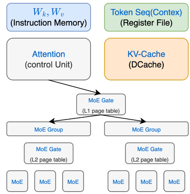
Then from the perspective of architecture, we want to increase the Cache hit rate as much as possible, which essentially requires cross-layer reuse of KVCache. And if we regard an integral Encoder/Decoder ( 1x Full + B x Reuse ) block as a recursive Transformer architecture, then the MoE of different layers exactly constitute different page tables. Next, based on this viewpoint, regard one layer of CSA2 as a small computer, and the three modes are the operation of the same set of data paths under three cache hit states.
By data lifecycle, one layer of CSA2 is divided into three architectural levels:
Compute (execution unit): the Main Q and SWA KV newly computed at each layer are local operands (like the register operands newly fetched by each instruction), and the main attention sparse_attnis the execution unit itself.Cache (on-chip shared cache): Main KV, Indexer K, TopK indices, and the HSI candidate pool are cross-layer shared reusable state, written by a certain source layer and read by multiple subsequent layers. Memory (large-capacity backend): the MoE / FFN of each layer is large-capacity storage and transformation, receiving the attention output.
Key correspondence: Main Q and SWA are always "newly fetched operands", never entering the shared cache; while Main KV / Indexer K / TopK are "cacheable state", whether to recompute depends on hit or miss.
Listing the read/write of the three types of shared state into an access pattern table:
| Mode | Main KV | Indexer K | TopK indices |
|---|---|---|---|
| Full | Write (fill) | Write (fill) | Write (compute) |
| Reindex | Read (hit) | Read (hit) | Write (recompute) |
| Reuse | Read (hit) | No access | Read (hit) |
Thus the three modes are exactly three cache states:
Full = write-back fill after cache miss (write-allocate): the execution unit computes all cacheable state and writes it, with the highest cost. Reindex = data hit, address recompute: the data (Main KV, Indexer K) hits, only the address generation is re-run to get new TopK, like a cache line resident but redoing one address translation. Reuse = full hit: both data and address hit, the execution unit only uses new operands (Main Q, SWA) to do one readout, which is the path closest to a pure load.
The Indexer of CSA2 corresponds to the CPU's address generation unit (AGU) and TLB: it does not move data, only produces the address set TopK of "which entries to read". The main attention is the data path, which fetches the Main KV from the shared cache by address and then computes.
Full: the AGU runs at full speed, scanning all causally visible positions to produce addresses, while filling data. Reindex: the data cache is resident, only restarting the AGU to re-translate addresses within a restricted range. Reuse: even the AGU is skipped, directly reusing the last address vector, which is equivalent to doing common subexpression elimination (CSE) and result memoization on the expensive address computation.
Decoupling of address generation and data path The HSI candidate pool is a TLB or working-set constraint. Layer 20 selects 2048 blocks totaling 16384 positions, which is equivalent to establishing a page table with a limited addressable range for the subsequent Reindex layers: the address recomputation of Reindex can only fall within the covered page (), and positions outside the pool are simply not addressable. The two-level TopK (block first, then position) is exactly a two-level page table: first use the block-level maximum score to select pages, then select specific entries within the page.
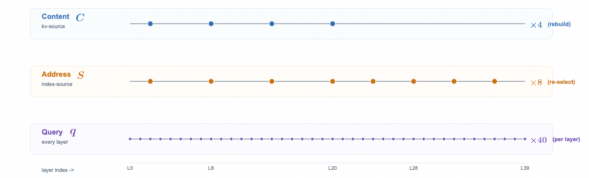
Three clock domains: usually we can regard Q as a query, the sparse selection such as TopK as an address, and the Main KV as content (a more precise definition refers to the next section). In fact, the three modes of CSA2 constitute three refresh timescales (content ×4, address ×8, query ×40) like three clock domains or the different refresh rates of three levels of storage: the query is register-level updated every cycle, the address is L1-level medium-frequency refill, and the content is L2/L3-level low-frequency refill. The closer to the execution unit, the faster and cheaper the refresh; the closer to the shared backend, the slower and more expensive the refresh. The mode scheduling of CSA2 is exactly placing each type of state at a refresh rate matching its recomputation cost.
3.3 The mathematical principle of cross-layer KV sharing
3.3.1 The three types of degrees of freedom of attention (content, address, query)
As introduced in 《On the Future Transformer: Loops Are Not What You Need》, for a transformer block, the injectable surfaces are: residual , the gain and bias of normalization, the metric , the bias , the summation range , the head set , the output gate, and the subsequent FFN. A figure summarizing them is as follows:
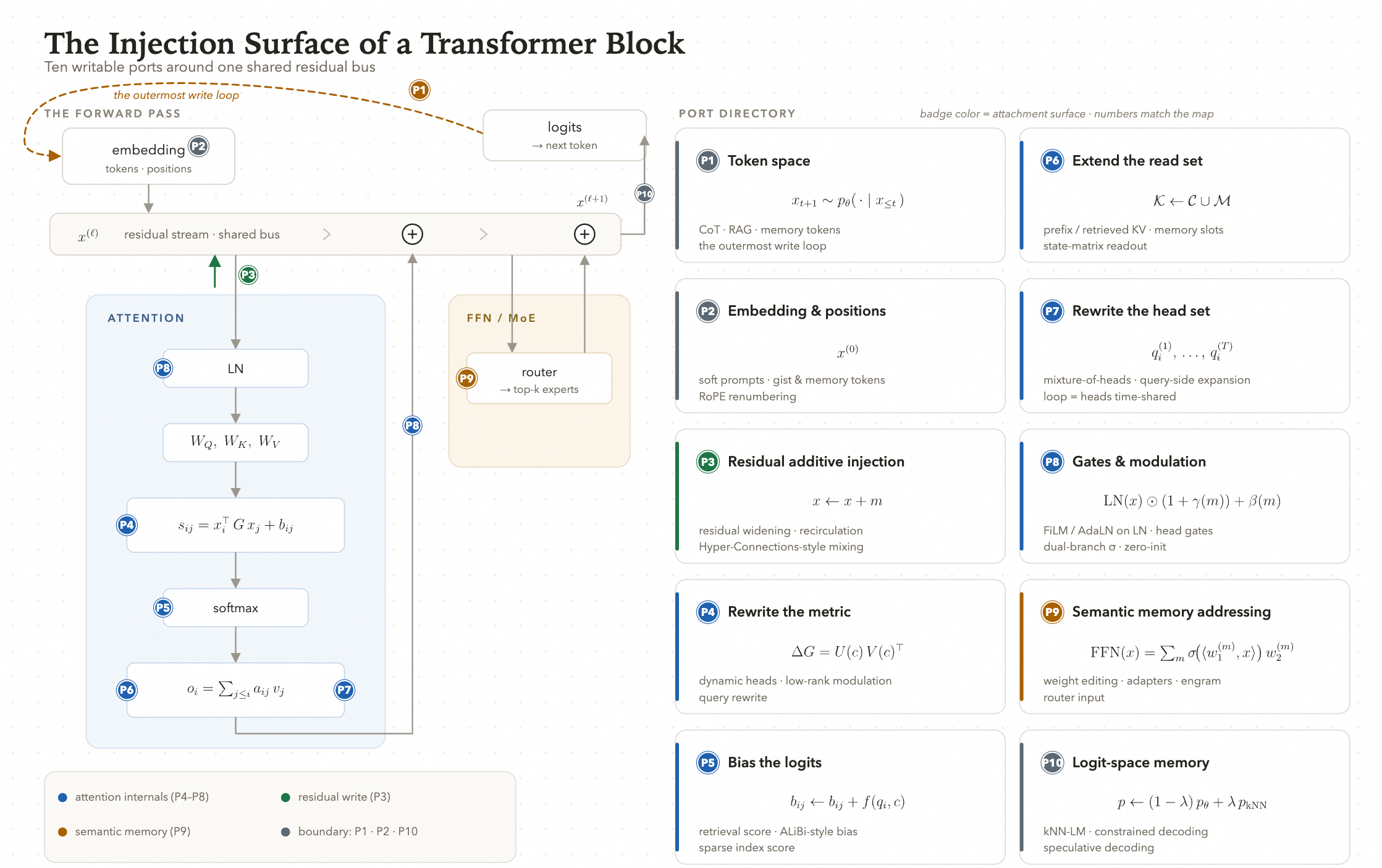
For Sparse Attention, any single sparse attention readout is essentially determined only by three variable inputs. Write the readout at query position as
The three variable inputs play non-overlapping roles.
Content is a set of content vectors obtained after compressing the history. In the reference implementation, the same simultaneously serves as K and V (key = value = ): when computing weights it acts as the Key, appearing in the inner product of the exponent; when producing the result it acts as the Value, appearing in the weighted sum . So the content decides two things at once, how similar an entry is to the query, and what is read out after a hit (the readout payload); this is different from standard attention, which splits K and V into two sets of projections. The address decides which content vectors this summation is normalized over, i.e., which positions to read from; The query decides the weight direction among these vectors. The output is a weighted average (convex combination, also called the barycenter) of the selected content vectors, falling within the convex hull they span. Content, address, and query, these three are the "three types of degrees of freedom of attention".
The definition, mathematical type, semantic role, and generation cost of the three types of degrees of freedom are each different.
Content : what to read (readable dictionary)
Definition: , generated by the gated pooling compressor at the kv-source layer over all published main entries. In the reference implementation key = value = . Type: continuous tensor , smooth and differentiable; it is the vertex set of the convex hull where the output lies. Role: "what to read". Content provides the retrievable semantic carrier; without it, both address and query lose their pointing target. Cost: most expensive. The compressor must scan all visible history, which is -level global computation.
Address : where to read from (sparse addressing)
Definition: , selected after the Indexer scores the candidates. Type: discrete combinatorial object , ; non-differentiable (TopK has zero gradient almost everywhere). Role: "where to read from". The address restricts the readout to normalize only over the selected content vectors, i.e., which vertices of the convex hull are chosen. Cost: medium. The Indexer needs to score the candidate set: the Full layer scans all causally visible positions, the Reindex layer only scans the candidate pool (at most ).
Query : how to read (readout direction)
Definition: , computed at each layer by the layer's own parameters from the current hidden state Type: continuous vector , smooth and differentiable. Role: "how to read". After is fixed, the query determines the weight distribution , i.e., the readout direction among the selected content vectors. Cost: cheapest. It is just the layer's own projection of the current hidden state, per-token , without scanning the history.
The threefold asymmetry of these three is the fulcrum of the entire CSA2 design:
Continuous vs discrete: are continuous and differentiable, is discrete and non-differentiable. Training gradients can only flow along ; can only be learned by an independent distillation path with the main attention as the teacher (Part four). Local vs global: is the layer's own local projection, must compress the global history, and must score all candidates. In generation cost, . Fast-changing vs slow-changing: the semantic content of the history changes slowest across layers, the address worth attending to drifts at medium speed, and the readout direction of each layer changes fastest.
The three also have a one-way dependency chain. The address is obtained by the Indexer scoring the content, so depends on ; the query is injected at the readout end only after is given to determine the weights. Denoted as
Therefore reuse can only proceed top-down along the dependency chain: one can reuse the content and jointly reuse the address (Reuse), one can reuse the content but reselect the address on the same content (Reindex), but one cannot change the content while reusing the old address. So the three modes of CSA2 are exactly three choices of "which degrees of freedom to refresh":
| Mode | Content | Address | Query | Refreshed degrees of freedom |
|---|---|---|---|---|
| Full | Newly computed | Newly selected (full scan) | Newly computed | All three refreshed |
| Reindex | Reused | Newly selected (within pool) | Newly computed | Address + query |
| Reuse | Reused | Reused | Newly computed | Query only |
3.3.2 The Reuse mode is based on query perturbation
Fix a layer , denote its input hidden state as , and a single token as . The main attention of one layer of CSA2 requires four tensors: Main Q, Main KV content, Top-K selection set, and local SWA KV. Below we first give the definition of each one by one, then prove that the reuse mode freezes three of them, leaving only the query variable.
Main Q is computed by the layer's own parameters from the current hidden state, consistent across the three modes:
Where is the RoPE of position , acting only on the rope tail channels, and each layer has its own independent .
Main KV content is generated only at the kv-source layer by the compressor ; is gated pooling, degenerating into a per-token projection when :
Top-K selection set is generated only at the index-source layer by the Indexer , where is the Indexer query, and is the per-head weight:
Local SWA KV is newly computed at each layer:
Readout concatenates the SWA and the selected Main KV into a single joint sparse attention:
Where .
Introduce two source mappings: is the Main KV source of layer , and is its index source; when the layer generates them itself, take or . Using the indicators and , write the content and selection uniformly as piecewise functions:
The three modes are exactly the value combinations of this pair of indicators:
That is, Full simultaneously newly generates content and selection, Reindex reuses content but regenerates selection, and Reuse reuses both; for the reuse layer , both content and selection are taken from an earlier source layer, independent of the layer's own hidden state , so their partial derivatives with respect to are zero:
Substituting these two zero partial derivatives back into the readout mapping, the dependency of on the layer's own input decomposes into two fresh channels plus two frozen constants:
For the frozen global memory , the only channel carrying the dependency is the query ; SWA is another independent fresh local channel, reconstructed layer by layer according to the fixed 128 window, without touching the global memory. Therefore, the inter-layer adaptation of the reuse layer to the global memory mathematically contracts exactly into one query rewrite
Where is the baseline query used by the index source layer when publishing the selection, and is the learnable perturbation of this layer. This is exactly the object of the subsequent expansion analysis.
3.3.2.1 The main attention can be written as a readout of a fixed dictionary
Let the candidate set of the reuse layer be , and stack the reused cache vectors by rows into . Because key = value = , the attention output is
Since is a family of non-negative weights summing to , the output is a convex combination of the dictionary vectors . Therefore
The output is locked in a convex polytope with fixed vertices, and rewriting can only move its position within that convex hull.
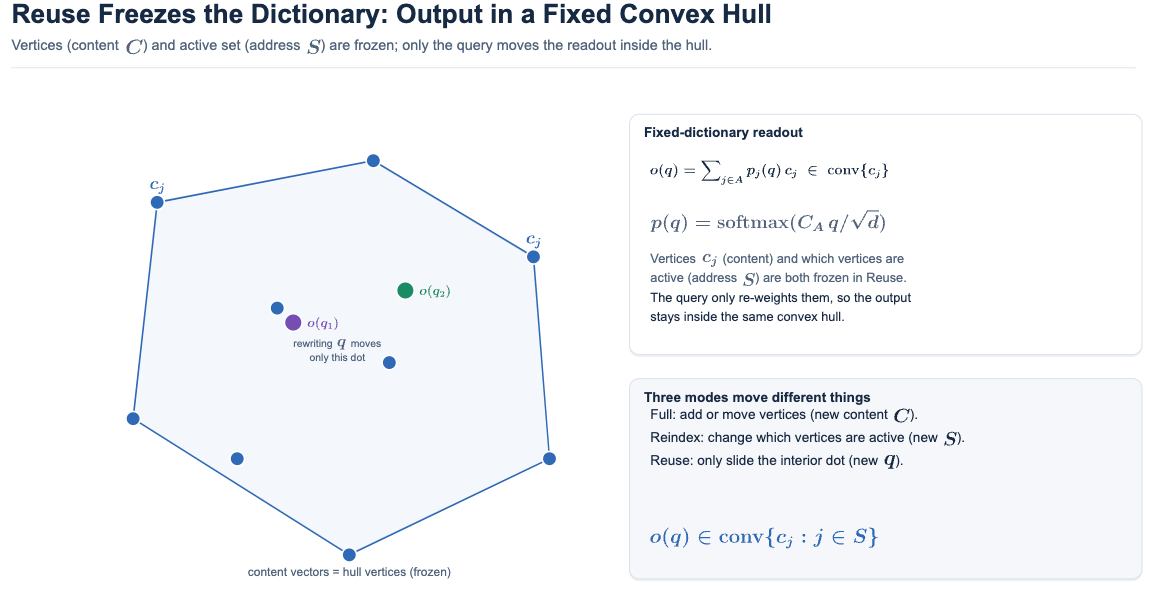
The next question to answer is: how large a range of this convex hull can moving actually cover?
In the DeepSeek-V4.1-Flash configuration, (head_dim), (sliding_window), (index_topk), so the candidate set size .
3.3.2.2 Rewriting Q is equivalent to exponential tilting of the baseline distribution
Denote the source layer's query as , and the baseline distribution . Any query of the reuse layer can be written in perturbation form . Substituting into (D1), the logit only gains one extra term , so
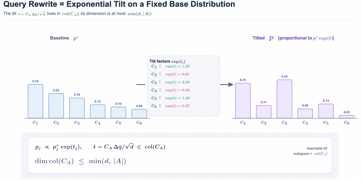
This shows that the query perturbation does one exponential tilting of the baseline distribution along the direction and then renormalizes. The achievable set of tiltings is
If (requires ), then any reweighting is reachable. In the DeepSeek-V4.1-Flash configuration, , so the tilting is restricted to a subspace of at most dimensions.
3.3.2.3 How large a range can the reuse output cover
Let the dictionary vectors be (i.e., the rows of , ), the base weights (i.e., the baseline distribution , satisfying ), and the scaling constant . Denote the query as a whole by (absorbing the merger of and ), define
is exactly the attention weight in (D1), and is the log partition function needed for its normalization. The attention output is denoted as the mean map
Thus the question of "how large a range the output can cover" can be seen as "what is the image set of the mean map ". When the query can freely traverse , or its effective linear subspace , and , the image of the mean map is
However, this is an capability upper bound, it describes "what can be reached at most if the query is completely free". But the real model's normalization, shared query bottleneck, and finite parameters do not guarantee access to all .
3.3.2.4 The expressiveness of only rewriting Q
So why does this query perturbation still have strong expressiveness when the Main KV is frozen?
Preserving the entire attention simplex. Within the range allowed by the rank, the reuse layer can still concentrate the mass onto a single selected entry (approaching a certain vertex), flatten it, or do arbitrary soft interpolation. Sharing the address is not equal to sharing the output. Fully differentiable, zero re-retrieval cost. The tilting is smooth with respect to , the gradient flows back normally, and each layer can specialize its way of reading the same memory; the skipped Indexer scoring and the non-differentiable TopK are not repeated. Geometric alignment. key = value = , increasing simultaneously raises the weight of and pulls the output toward , and the perturbation is a directly interpretable control of the output position. The global-vs-local ratio is also managed by . SWA and Main KV are in the same softmax, and also allocates the mass between the frozen global memory and the fresh local window.
Another potential speculation is that we can, through some kind of learnable Q-aware parameters, map the KV space of the next layer back to the current layer to achieve reuse.
Specifically, in a standard Transformer, the KV of each layer changes with the residual, thus constituting a manifold of a high-dimensional space in the layer dimension. Then is there a situation where, separating out , using this information as some kind of spatial mapping, especially when mHC can maintain a relatively stable residual, so that the space constituted by the KV of the later layer can be mapped back to the space constituted by the KV of the earlier layer through some Q-aware parameter weights, and let the model absorb this spatial mapping information into MoE/FFN and Engram during the training stage.
In this way, the KV can be fixed, while the Q-aware parameter mapping maps it to an appropriate position? Even if there are some defects that cannot be remedied, is it possible to convert these defects from the layer dimension of the model into a longer sequence dimension, for example a new fixed KV space constituted by some special CoT to represent it?
This content is recorded in some internal documents, and related experimental analysis is being carried out.
3.3.2.5 The difference between Reuse and Full modes
The Full layer has three degrees of freedom that vary independently per layer:
| Degree of freedom | Full | Reuse |
|---|---|---|
| (F1) Query | Yes | Yes, uniquely retained |
| (F2) Key-value content , moving polytope vertices and changing the tilting geometry | Yes | No, frozen |
| (F3) Selection set , which vertices exist, discrete | Yes | No, frozen |
For fixed memory there is strict inclusion , and Full also takes the union over all . The expressiveness gap is exactly the three things reuse cannot do:
Recall upper bound: content with is not in , no can reach it, and an upstream TopK selection error cannot be corrected downstream. Vertices immovable: the output is nailed within the fixed convex hull , and Full changing can place the output outside the convex hull. Tilting geometry unswappable: the reachable distribution of reuse is a fixed exponential family determined by , and Full reselecting is equivalent to replacing the entire family.
In addition, RoPE only applies a position-dependent orthogonal rotation to the rope tail of and , which is absorbed into the inner product , and does not change the above convex hull and tilting argument.
3.3.3 The synergy of Full / Reindex / Reuse
In the dimension of the model layers, the three modes constitute the following structure:
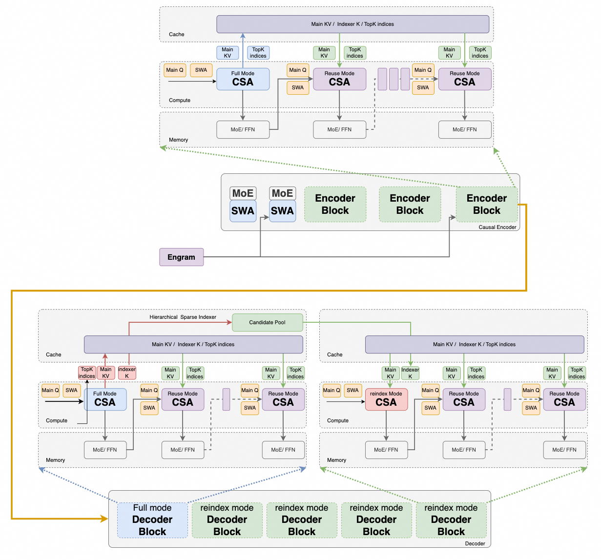
The three modes constitute a coarse-to-fine refresh schedule, corresponding to three timescales:
Full rebuilds the KV cache, runs the complete Indexer plus TopK, and is the anchor. Reindex retains the content, re-scores and reselects Top-K within the HSI candidate pool, and does not rebuild the KV. Reuse only does Q projection, SWA, and one sparse_attn, without scoring, without TopK, and without writing KV.
In the Decoder, HSI is also introduced, so the division of labor of the three modes in the decoder is:
Full, denoted (layer 20): defines the content , defines the candidate pool (16384 positions), and gives its own Top-512. Reindex, denoted (24, 28, 32, 36): the content is unchanged, reselects each of their own Top-512 within , i.e., . Reuse, denoted : follows the published by the most recent index layer, only rewriting the query.
DeepSeek-V4.1-Flash:Pushing the Limits of KV Cache Compression: https://huggingface.co/deepseek-ai/DeepSeek-V4.1-Flash/blob/main/DeepSeek_V41_Tech_Report.pdf
[2]You Only Cache Once:Decoder-Decoder Architectures for Language Models: https://arxiv.org/pdf/2405.05254
[3]Building Effective Sparse MoE Models with Moderate Resources: https://welm.weixin.qq.com/en/posts/building-effective-sparse-moe-models-with-moderate-resources/#kv-mirror
[4]PowerAttention: Exponentially Scaling of Receptive Fields for Effective Sparse Attention: https://arxiv.org/abs/2503.03588
[5]Reducing Transformer Key-Value Cache Size with Cross-Layer Attention: https://proceedings.neurips.cc/paper_files/paper/2024/file/9e23d020c18e4c40d81c6a0fc7a46f68-Paper-Conference.pdf
[6]IndexCache: Accelerating Sparse Attention via Cross-Layer Index Reuse: https://arxiv.org/abs/2603.12201
[7]You Only Index Once: Cross-Layer Sparse Attention with Shared Routing: https://arxiv.org/pdf/2606.06467
[8]HySparse: A Hybrid Sparse Attention Architecture with Oracle Token Selection and KV Cache Sharing: https://arxiv.org/pdf/2602.03560
[9]HISA: Efficient Hierarchical Indexing for Fine-Grained Sparse Attention: https://arxiv.org/pdf/2603.28458v1